an epoch, a single training loop over all training data instances, costs O n2 , where n is the number of training data points. (View Highlight)
Note: I have no idea where he’s getting this from. If it cost O(n^2) just to compute the loss, large models would be completely intractable.
The loss of observation does not depend on the loss of any other observation. The loss computation for one observation is O(1). The loss computation for all observations is the sum of all of these, O(n).
Let us define as some measure of the “size” of the network. ( is encapsulating a lot of complexity, but the point is that it’s not dependent on the number of observations ). The total computational complexity of an epoch is:
Forward propagation of all observations through the network, ;
The computation of the loss for each observation, ;
The backpropagation of the loss through the network, .
The complexity of the epoch overall is dominated by the forward propagation step, so the time complexity of an epoch is , where is invariant to the size of the dataset and typically much smaller than .
So just no.
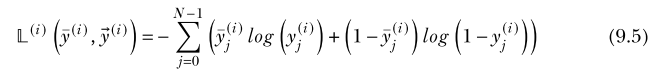
Note: Binary cross-entropy loss. Derive this from the general formula for cross-entropy loss in my notes.
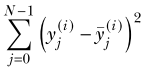
Given a pair of normalized tensors (such as images or vectors) whose elements all have values between 0 and 1, a variant of the two-class CE loss can be used to estimate the mismatch between the tensors. (View Highlight)
Note: When comparing two images, such as the input and output of an autoencoder, we can sum the binary cross-entropy loss from each pixel and channel to provide a total binary cross-entropy loss for the whole image.
New highlights added June 26, 2024 at 2:00 PM
it is desirable to make the last layer of a classifier neural network a softmax layer. Then, given an input, the network will emit probabilities for each class. (View Highlight)
the softmax is often followed by the CE loss during classifier training. Consequently, the combination (softmax CE loss) is available as a single operation in many deep learning packages, such as PyTorch. (View Highlight)
Softmax CE loss is probably the most popular loss method used for training in classifiers at the moment. (View Highlight)
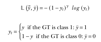
To stop focusing on easy examples and focus instead on hard examples, we can put more weight on the loss from training data instances that are far from the GT, and vice versa: that is, put less weight on the loss from training data instances that are close to GT. (View Highlight)
Note: The focal loss proceeds from the case where we use binary cross-entropy loss. In binary cross-entropy loss, one term always cancels out. Focal loss continues from this and adds adds a term that reflects the magnitude of the deviation of the softmax prediction for the ground truth label. Exponentiating this term by a tunable parameter gives the focal loss.
Sometimes we prefer to stop changing the network when the correct class has the maximum score, and we do not care about increasing the distance between correct and incorrect scores any further. (View Highlight)
a hinge loss function increases if a certain goodness criterion is not satisfied but becomes zero (and does not reduce any further) if the criterion is satisfied. (View Highlight)
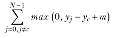
multiclass support vector machine (SVM) loss (View Highlight)
Note: He forgot to actually define hinge loss, which is for binary classification problems and is defined as
The generalization of hinge loss to multiclass classification is called the SVM loss, also known as the Crammer-Singer loss:
Note: The extensive failure to use \mathrm in this chapter, along with forgetting to include the equation for hinge loss and giving this inexplicable nonsense about calculating loss for an epoch taking time reflects a serious lack of editing in this chapter.
Note: For hinge loss (and its multiclass generalization, SVM loss), the incorrect label’s logit (not probability) is smaller than the correct label’s logit by at least a margin of . If it is not, it contributes to the loss.
When using hinge/svm loss, you need to use it on the raw scores (logits).
The loss is zero in “easy” cases (those classified beyond the margin ). As such, the gradient is zeroed out for all of these cases as well. This means that all parameter adjustments are based on cases that are either misclassified or classified with low confidence (within the margin). This may be a good thing or a bad thing, but it’s usually a bad thing because it makes it much slower and harder to converge.
Situations where it’s potentially useful:
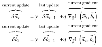
Note: SGD with momentum takes a weighted average of the current gradient and the last update (“velocity”).
Notice that the velocity vector at . Hence the first update is “slower” than it would otherwise have been (by a factor of ). Technically, this slowness persists throughout training, decaying exponentially over the subsequent updates. Of course, it’s completely negligible after a small number of updates.
Note: Using the Taylor expansion, we see that the total contribution of prior velocities to the current approaches \mathbf{\eta}{1 - \gamma}\t \rightarrow \infty$.
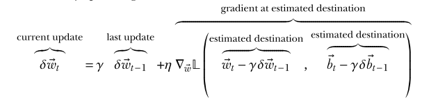
Note: Nesterov’s accelerated gradient (NAG) computes the gradient with respect to the CURRENT weights of a point in parameter space described by the CURRENT weights offset by the the CURRENT momentum (which is a fraction of the weight changes in the PREVIOUS iteration). This is scaled by the learning rate and added to an ordinary momentum term.
At , this looks like ordinary SGD: we are taking the gradient, with respect to the weights, of the loss evaluated given the current parameter values and \mathbf{b}$. The momentum term is zero, and the offset is zero.
During the forward pass, NAG uses the “look-ahead” parameters (current parameters offset by momentum) instead of the actual current parameter values.
NAG behaves more or less like ordinary momentum unless the current momentum would cause the parameters to overshoot the optimum. If this happens, the gradient given the look-ahead parameters will have the opposite sign as the momentum term, so a weighted sum cancel each other out to a (tunable) degree.
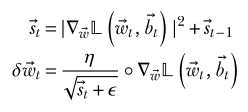
Note: AdaGrad maintains a state vector consisting of the sum over all iterations of the squared partial derivatives of each parameter in the model. That is, if is the state vector at time , then the value for parameter is
Note that the norms shown in Chaudhury’s version here are misleading, though not technically incorrect because these partials are real scalars. Though honestly, I’m getting sick and tired of tolerating these mistakes.
Hadamard operator (elementwise multiplication ofthe two vectors) (View Highlight)
A significant drawback of the AdaGrad algorithm is that the magnitude of the vector st keeps increasing as iteration progresses. This causes the LR for all dimensions to become smaller and smaller. (View Highlight)
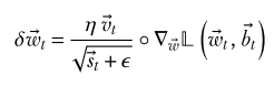
Note: RMSProp adds an additional parameter that effectively changes the state vector from a sum of past states to an exponential moving average of them. Larger values of extend the number of previous states that make a non-negligible contribution.
after many iterations, the RMSProp state vector effectively takes the weighted average ofthe past term-wise squared gradient magnitude vectors (View Highlight)
 (View Highlight)
 (View Highlight)
 (View Highlight)
 (View Highlight)
 (View Highlight)
 (View Highlight)
 (View Highlight)
 ?t=1719432226045 (View Highlight)
 (View Highlight)
 (View Highlight)
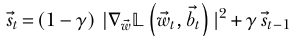 (View Highlight)
 (View Highlight)