David’s summary
While there is some dispute about its priority, this very short (~2 pages) paper is unquestionably the one that brought modern neural networks to the fore. It builds on the Single-layer perceptron, which functions similarly but has pre-specified weights.
In plain and accessible language, the paper introduces the concept of backpropagation, which makes it possible to train a neural network from random initial weights. The bulk of the discussion focuses on the derivation of, and two strategies for using, the method.
Following this, they briefly touch on a couple of examples of feed-forward neural network. They foreshadow a couple of interesting ideas: that higher-order effects (like symmetry) require more than just an input and an output layer; and that it is possible to use the same strategy to create a recurrent neural network, though they do not explore this.
The paper is frustratingly light on exactly how to implement a training loop using gradient descent and backpropagation, so Claude AI and I wrote an annotated version in Python.
Readwise
Metadata
- Full Title: Learning representations by back-propagating errors
- Category:articles
- URL: https://readwise.io/reader/document_raw_content/33063543
Highlights
- more difficult when we introduce hidden units whose actual or desired states are not specified by the task. (View Highlight)
- The simplest form of the learning procedure is for layered networks which have a layer of input units at the bottom; any number of intermediate layers; and a layer of output units at the top. (View Highlight)
- connections can skip intermediate layers. (View Highlight)
- Note: In this original paper, direct connections from a layer to a future non-neighbor is permitted. This is no longer common, but apparently still happens (eg in ResNet).
- As a result of the weight adjustments, internal ‘hidden’ units which are not part of the input or output come to represent important features of the task domain, and the regularities in the task are captured by the interactions of these units. (View Highlight)
- Learning becomes more interesting but (View Highlight)
- (2) (View Highlight)
- Note: Original activation function was a simple sigmoid
- there is a fixed, finite set of input-output cases, the total error in the performance of the network with a particular set of weights (View Highlight)
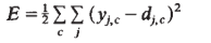
- The aim is to find a set of weights that ensure that for each input vector the output vector produced by the network is the same as (or sufficiently close to) the desired output vector. If there is a fixed, finite set of input-output cases, the total error in the performance of the network with a particular set of weights can be computed by comparing the actual and desired output vectors for every case. The total error, E, is defined as (View Highlight)
 (View Highlight)
- Note: The total error is the sum over all cases and output units of the squared error.
- gradient descent (View Highlight)
- Note: The idea of optimizing a function by moving in the direction of steepest gradient dates back to the early 19th century.
New highlights added April 11, 2024 at 11:56 AM
- The backward pass starts by computing aE/ay for each of the output units. (View Highlight)
- (4) (View Highlight)
- Note: By “suppressing the index
,” they mean we should understand eq 4 as: ∂E_c/∂y_{j,c} = y_{j,c} - d_{j,c} Which is to say, we should interpret equation (4) to mean: “The change in the error for case as a function of a change in the value of output unit for case is the difference between that value and the true value.”
- Note: By “suppressing the index
- (6) (View Highlight)
New highlights added April 11, 2024 at 1:55 PM
- Yi, of the units that are connected to j and of the weights, wii• on these connection (View Highlight)
- (1) (View Highlight)
- (5) (View Highlight)
New highlights added April 11, 2024 at 2:56 PM
- utput cases, For a given case, the partial derivatives of the err (View Highlight)
New highlights added April 11, 2024 at 9:14 PM
- ( (View Highlight)
- this total input is just a linear function of the states of the lower level units and it is also a linear function of the weights on the connections, so it is easy to compute how the error will be affected by changing these states and weights. (View Highlight)
- (7) (View Highlight)
New highlights added April 12, 2024 at 9:43 AM
- O (View Highlight)
- Note: They propose two ways to update the weights during training: update after every observation, or sum all the errors and update after processing all observations.
- (8) (View Highlight)
- Note: The simplest thing to do is just to multiply accumulated error by some learning parameter
and adjust the weight by that much.
- Note: The simplest thing to do is just to multiply accumulated error by some learning parameter
- using an acceleration method in which the current gradient is used to modify the velocity of the point in weight space instead of its position (View Highlight)
- a is an exponential decay factor between O and 1 that determines the relative contribution of the current gradient and earlier gradients to the weight change. (View Highlight)
New highlights added April 12, 2024 at 10:47 AM
- Adding a few more connections creates extra dimensions in weight-space and these dimensions provide paths around the barriers that create poor local minima in the lower dimensional subspaces. (View Highlight)