Summary: Deep learning uses backpropagation to uncover complex patterns in data through multiple layers of representation. These deep neural networks can learn to distinguish important features and filter out irrelevant information. Recent advancements in deep learning have led to applications in various fields like computer vision and natural language processing.
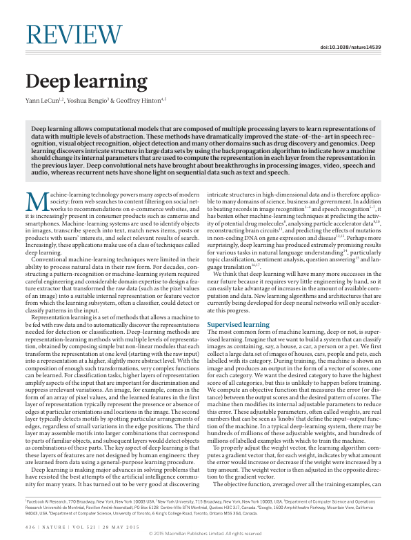
Note: The change in error with respect to the activation of node does not depend directly on the activation of the nodes in the next layer . Rather, it has a direct dependence only on the summed inputs of that node and the weight between them, since that’s how those two nodes interact. However, still depends indirectly on , because depends on via the chain rule.
A multi- layer neural network (shown by the connected dots) can distort the input space to make the classes of data (examples of which are on the red and blue lines) linearly separable. (View Highlight)
At each layer, we first compute the total input z to each unit, which is a weighted sum of the outputs of the units in the layer below. Then a non-linear function f(.) is applied to z to get the output of the unit. (View Highlight)
At each hidden layer we compute the error derivative with respect to the output of each unit, which is a weighted sum of the error derivatives with respect to the total inputs to the units in the layer above. We then convert the error derivative with respect to the output into the error derivative with respect to the input by multiplying it by the gradient of f(z). (View Highlight)
Note: What’s striking is how, even before the era of Transformers, we could get solid image-to-text results just by chaining together a CNN with an old-school generative RNN.
New highlights added June 22, 2024 at 9:58 AM
Deep learning discovers intricate structure in large data sets by using the backpropagation algorithm to indicate how a machine should change its internal parameters that are used to compute the representation in each layer from the representation in the previous layer. (View Highlight)
deep learning will have many more successes in the near future because it requires very little engineering by hand, (View Highlight)
Note: Not entirely true in 2024. First of all, network architecture design is not at all trivial, and new tricks (at ever-higher levels of abstraction) are being discovered all the time. More urgently, though, larger models quickly run into physical resource constraints, and a model is useless—no matter how powerful on paper—if you can’t actually use it.
For decades, con- structing a pattern-recognition or machine-learning system required careful engineering and considerable domain expertise to design a fea- ture extractor (View Highlight)
Representation learning is a set of methods that allows a machine to be fed with raw data and to automatically discover the representations needed for detection or classification. Deep-learning methods are representation-learning methods with multiple levels of representa- tion, (View Highlight)
Since the 1960s we have known that linear classifiers can only carve their input space into very simple regions, namely half-spaces sepa- rated by a hyperplane19 (View Highlight)
To make classifiers more powerful, one can use generic non-linear
features, as with kernel methods20
, but generic features such as those
arising with the Gaussian kernel do not allow the learner to general-
ize well far from the training examples21 (View Highlight)
this can all be avoided if good features can be learned automatically using a general-purpose learning procedure (View Highlight)
As it turns out, multilayer architectures can be trained by simple stochastic gradient descent. As long as the modules are relatively smooth functions of their inputs and of their internal weights, one can compute gradients using the backpropagation procedure. (View Highlight)
The backpropagation algorithm (Fig. 1) can be directly applied to the computational graph of the unfolded network on the right, to compute the derivative of a total error (for example, the log-probability of generating the right sequence of outputs) with respect to all the states st and all the parameters. (View Highlight)
Note: We have three weight matrices: the weights from input to hidden state; the weights from hidden state to hidden state; and the weights from hidden state to output. We’re going to update them by some flavor of gradient descent as usual.
The tricky thing to understand is how we get the gradient in the first place. The key is to realize that, once you’ve actually run an input through the RNN, there is a definite number of “layers.” If we assume that only the final hidden state is used for the output, then (in retrospect) the function as executed looks like a fully connected feedforward network, at least as far as backpropagation is concerned. We have a constraint that the weights must all match at the end of our parameter update, and they need to reflect the state of all of the layers.
The clues are in the constraint. If we need them to match, and we need them to reflect all the layers, we can just do the obvious and add up the gradient (change in error wrt inputs and outputs) at all the layers. And indeed, that is literally all there is to implementing backpropagation through time: We calculate the gradient of the loss from the prediction to the target at the output state, then backpropagate the gradient to the -th layer. We proceed as normal, calculating the gradient of the error with respect to the outputs and inputs of each layer. External to this, we accumulate the gradient value for each weight. We use this externally accumulated gradient to update the weights exactly as usual.
New highlights added June 22, 2024 at 5:05 PM
Once these gradients have been computed, it is straightforward to compute the gradients with respect to the weights of each module. (View Highlight)
Note: You don’t have to do this in the order specified.
For each layer , you have three gradients of interest:
The gradient of the loss wrt the output ;
The gradient of the loss wrt to the inputs ; and
The gradient of the loss wrt the weights .
The value of (1) for layer depends on the value of (2) for layer . But, although it’s the thing we ultimately need for SGD, nothing in the backprop process depends on (3), so we can do it whenever we like.
Note that all of these gradients are tensors. In the case of a CNN, where you may have multiple channels per pixel, you’re looking at a rank-3 weight tensor, and so a rank-3 tensor for .
The hidden layers can be seen as distorting the input in a non-linear way so that categories become linearly separable by the last layer (View Highlight)
Recent theoretical and empirical results strongly suggest that local minima are not a serious issue in general. (View Highlight)
New highlights added June 22, 2024 at 6:05 PM
Mathemati- cally, the filtering operation performed by a feature map is a discrete convolution, hence the name. (View Highlight)
The researchers intro- duced unsupervised learning procedures that could create layers of feature detectors without requiring labelled data. (View Highlight)
Note: This was achieved with Boltzmann Machines (BMs). Like autoencoders, BMs learn to reproduce the input data. The difference is in how they do it: autoencoders force the model to propagate the input through an information bottleneck, whereas BMs learn a statistical distribution through a network that has connections in both directions (not to be confused with a BiRNN, which has two sets of directed neurons in each layer).
BMs apparently are hard to work with and thus have achieved limited practical use, though a variant called Restricted Boltzmann Machines have real-world applications.
Although the role of the convolutional layer is to detect local con- junctions of features from the previous layer, the role of the pooling layer is to merge semantically similar features into one. (View Highlight)
Two or three stages of convolution, non-linearity and pool- ing are stacked, followed by more convolutional and fully-connected layers. (View Highlight)
Deep neural networks exploit the property that many natural sig- nals are compositional hierarchies, in which higher-level features are obtained by composing lower-level ones. (View Highlight)
Once deep learning had been rehabilitated, it turned out that the pre-training stage was only needed for small data sets. (View Highlight)
There was, however, one particular type of deep, feedforward net-
work that was much easier to train and generalized much better than
networks with full connectivity between adjacent layers. This was
the convolutional neural network (ConvNet)41,42
. (View Highlight)
There are four key ideas behind ConvNets that take advantage of the properties of natural signals: local connections, shared weights, pooling and the use of many layers. (View Highlight)
Note: I had never seen this term. Apparently, it’s just an older term for what we now call “filter.” Each filter produces a channel in the output of a layer.
New highlights added June 22, 2024 at 7:05 PM
When deep convolutional networks were applied to a data set of about a million images from the web that contained 1,000 different classes, they achieved spec- tacular results, almost halving the error rates of the best compet- ing approaches1. (View Highlight)
Deep-learning theory shows that deep nets have two different expo- nential advantages over classic learning algorithms that do not use distributed representations21 (View Highlight)
ConvNets are now the dominant approach for almost all recognition
and detection tasks4,58,59,63–65
and approach human performance on
some tasks. (View Highlight)
First,
learning distributed representations enable generalization to new
combinations of the values of learned features beyond those seen
during training (for example, 2n combinations are possible with n
binary features)68,69
. Second, composing layers of representation in
a deep net brings the potential for another exponential advantage70
(exponential in the depth). (View Highlight)
RNNs process an input sequence one element at a time, maintaining in their hidden units a ‘state vector’ that implicitly contains information about the history of all the past elements of the sequence. (View Highlight)
RNNs are very powerful dynamic systems, but training them has
proved to be problematic because the backpropagated gradients
either grow or shrink at each time step, so over many time steps they
typically explode or vanish77,78
. (View Highlight)
When trained to predict the next word in a news story, for example, the learned word vectors for Tuesday and Wednesday are very similar, as are the word vectors for Sweden and Norway. Such representations are called distributed representations because their elements (the features) are not mutually exclusive and their many configurations correspond to the variations seen in the observed data. (View Highlight)
This rather naive way of performing machine translation has quickly become competitive with the state-of-the-art, and this raises serious doubts about whether understanding a sen- tence requires anything like the internal symbolic expressions that are manipulated by using inference rules. (View Highlight)
Although we have not focused on it in this Review, we expect unsupervised learning to become far more important in the longer term. (View Highlight)
Instead of translating the meaning of a French sentence into an English sentence, one can learn to ‘translate’ the meaning of an image into an English sentence (Fig. 3). The encoder here is a deep Con- vNet that converts the pixels into an activity vector in its last hidden layer. The decoder is an RNN similar to the ones used for machine translation and neural language modelling. (View Highlight)
We expect
systems that use RNNs to understand sentences or whole documents
will become much better when they learn strategies for selectively
attending to one part at a time76,86
. (View Highlight)
Note: The use of the word “attend” here was not an extraordinarily lucky turn of phrase; they cite Bahdanau in this sentence
(LSTM) networks that use special hidden units, the natural behaviour of which is to remember inputs for a long time79 (View Highlight)
Note: Transformers didn’t fully kill off LSTMs, but they did largely supplant them in NLP. Today, LSTMs are largely used for time series data.
 (View Highlight)
 (View Highlight)