for large values ofw, the parameterized sigmoid is virtually indistinguishable from the Heaviside step function (View Highlight)
the derivative (gradient) of the function near x = 0 is much higher for tanh than for sigmoid. Stronger gradients mean faster convergence, as the weight updates happen in larger steps (View Highlight)
Why do extra layers help? The primary reason is the extra nonlinearity. (View Highlight)
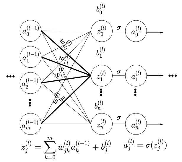
Such a layer is also known as fully connected layer. (View Highlight)
Note: Linear layers are synonymous with fully connected layers. Note, however, that this has no implication about the activation function of the neurons. This is because the activation function is often modeled as a separate “layer.”
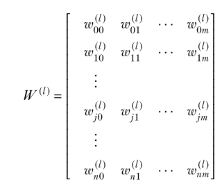
The weight of the connection from the kth neuron in layer (l −1) to the jth neuron in layer l is denoted w(l ) jk . (View Highlight)
Note: In this weight matrix , the rows correspond to target neurons in layer , and the columns correspond to source neurons in layer . The row index is and the column index is . We write an entry as .
The final output of an MLP with fully connected (aka linear) layers 0 · · · L on input x can be obtained by repeated application of this equation (View Highlight)
Note: A neural network can be understood as the composition of the linear combination and activatiion functions for each layer.
The complicated equation 8.9 is never explicitly evaluated. Instead, we evaluate the outputs of successive layers, one layer at a time, as per equation 8.10. Every layer can be evaluated by taking the previous layer’s output as input. No other input is necessary. (View Highlight)
New highlights added June 25, 2024 at 4:45 PM
In general, if a loss, denoted 핃, is expressed as a function of the parameters, such as 핃 w, b , then the change in the parameters that optimally takes us toward lower loss is yielded by the gradient of the loss with respect to the parameters ∇w,b핃 w, b . (View Highlight)
Note: I find this unhelpful, as it just makes the equations below harder to read (since I have to keep going back and checking what means).
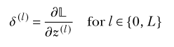
I think the idea is that, in implementing this, you need to keep track of , and maybe people usually call this “deltas.”
That said, it’s not really an “auxiliary variable” in the sense that we usually use them: as a substitution that allows us to complete a mathematical analysis that otherwise would run into trouble during intermediate steps.
Note: Again, the insistence on MSE as “the loss” makes me wonder how worthwhile it is to read this carefully. The analysis also depends explicitly on the sigmoid activation function, but at least he’s upfront about that.
 (View Highlight)
 (View Highlight)
 (View Highlight)