Summary: The text discusses implementing a dataset object in PyTorch for feeding data into a model and training modern neural networks. It covers topics like implementing training loops, changing loss functions, and optimizing neural networks using smaller data batches. PyTorch provides tools like Dataset abstraction to simplify tasks and improve memory usage during training.
The main exception to using 32-bit floats or 64-bit integers as the dtype is when we need to perform logic operations (like Boolean AND, OR, NOT), which we can use to quickly create binary masks.
A mask is a tensor that tells us which portions of another tensor are valid to use. (View Highlight)
x = x.to(device) time_gpu = timeit.timeit(”x@x”, globals=globals(), number=100) (View Highlight)
Note: Move your computation to the GPU
this only works if every object involved is on the same device. (View Highlight)
you will often see code that looks like x.cpu().numpy() when you want to access the results of your work. (View Highlight)
The .to() and .cpu() methods make it easy to write code that is suddenly GPU accelerated. Once on a GPU or similar compute device, almost every method that comes with PyTorch can be used and will net you a nice speedup. (View Highlight)
The second major foundation that PyTorch gives us is automatic differentiation: as long as we use PyTorch-provided functions, PyTorch can compute derivatives (also called gradients) automatically for us. (View Highlight)
The sign of the gradient f tells us which direction we should move to find a minimizer. (View Highlight)
. Once we tell PyTorch to start calculating gradients, it begins to keep track of every computation we do. It uses this information to go backward and calculate the gradients for everything that was used and had a requires_grad flag set to True. (View Highlight)
Once we have a single scalar value, we can tell PyTorch to go back and use this information to compute the gradients. This is done using the .backward() function, after which we see a gradient in our original object (View Highlight)
PyTorch includes two additional concepts to help us: parameters and optimizers. A Parameter of a model is a value that we alter using an Optimizer to try to reduce our loss (·). (View Highlight)
Note: Refer back to the PDF (PDF p58, text p24) to capture the code that maps PyTorch’s optimizer to a manual while loop
The simplest optimizer we use is called SGD, which stands for stochastic gradient descent. (View Highlight)
To use SGD, we need to create the associated object with a list of Parameters that we want to adjust. We can also specify the learning rate η or accept the default. (View Highlight)
PyTorch sits at a better balance between “make things easy” and “make things acces- sible” than most of the other tools. The NumPy-like function calls make development fairly easy and, more importantly, easier to debug. While PyTorch has nice abstractions like the Optimizer, we have just seen how painless it is to switch between different levels of abstraction. (View Highlight)
PyTorch is also flexible for use outside classical deep learning tasks. (View Highlight)
In many cases, we need to do non-trivial preprocessing, preparation, and conversions to get our data into a form that a neural network can learn from. If you put those tasks into the getitem function, you get the benefit of PyTorch doing the work on an as-needed basis while you wait for your GPU to finish processing some other batch of data, making your overall process more compute efficient. (View Highlight)
for any situation where int types are required, PyTorch is hardcoded to work only with int64, so you just have to use it. (View Highlight)
PyTorch has a simple utility to break the corpus into train and test splits. Let’s say we want 20% of the data to be used for testing. We can do that as follows using the random_split method: (View Highlight)
New highlights added May 30, 2024 at 4:24 PM
The vector of weights that makes a logistic/linear regression is also called a linear layer or a fully connected layer. This means both can be considered a single layer model in PyTorch. (View Highlight)
a process called a training loop with three major components: the training data (with correct answers), the model and loss function, and the update via gradients. (View Highlight)
The three major steps to training a model in PyTorch. 1. The input data drives learning. 2. The model is used to make a prediction, and a loss scores how much the prediction and true label differ. 3. PyTorch’s automatic differentiation is used to update the parameters of the model, improving its predictions. (View Highlight)
y ˆy = fΘ(x) to state that the model’s prediction and behavior depend on the value of its parameters Θ. You will also see Θ called the state of the model. (View Highlight)
The loss function quantifies how badly our model is doing at the goal of predicting the ground truth y. If y is our goal and ˆy is the prediction, we will denote our loss function as (ˆy, y). (View Highlight)
Suppose Θk is the current state of our model, which we want to improve. How do
we find the next state Θk+1, which hopefully reduces our model’s loss? The equation
we want to solve is Θk+1 = Θk − η ·
1 N
N
i=1 ∇Θk(fΘk
(xi), yi). (View Highlight)
A common convention in some ML research: when you have a larger function to optimize that is composed of the total loss over many smaller items, denote the larger function as F and the inner function as f. (View Highlight)
We need an iterator that loads the training data for us to train on.2 This training_loader will gives us pairs of inputs with their associated labels for training. (View Highlight)
Note: Accumulate a running loss within the epoch, but reset it at the start of each new epoch. Nevertheless, use only the loss from the current batch to update (“step”) the parameters.
The standard approach is to pick the data points at random one at a time, which ensures that your model learns the data and not the order of the data. (View Highlight)
while your model is busy training on the GPU, your DataLoader is busy fetching the next data so the GPU is as busy as possible. (This type of performance optimization is often called pipelining.) (View Highlight)
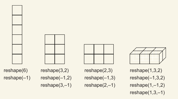
What is special about reshape is that it lets us specify all but one of the dimensions, and it automatically puts the leftovers into the unspecified dimension. This leftover dimension is denoted with –1 (View Highlight)
The vector x has all of our d features (in this case, d = 1), and the matrix W has a row for every feature and a column for every output. We use Wd,C to be extra explicit that it is a tensor with d rows and C columns. (View Highlight)
Note: Linear regression
we add a bias term b that has no interaction with x (View Highlight)
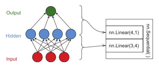
nn.Linear(d, C). This creates a linear layer with d inputs and C outputs (View Highlight)
Because bias terms are almost always used but are annoying and cumbersome to write out, they are often dropped and assumed to exist implicitly. (View Highlight)
Modules are how PyTorch organizes the building blocks of modern neural network design. Modules have a forward function that takes inputs and produces an output (we need to implement this if we make our own Module), and a backward function (PyTorch takes care of this for us unless we have a reason to intervene). (View Highlight)
You have two loss functions, L1 and MSE, both of which are appropriate for a regres- sion problem. (View Highlight)
if the problem you are trying to solve is one where small differences are OK but large ones are really bad, the MSE loss might be a better choice. If your problem is such that being off by 200 is twice as bad as being off by 100, the L1 loss makes more sense. (View Highlight)
for any computation done within the scope of the no_grad() block, do not calculate gradients (View Highlight)
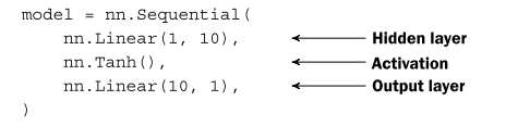
Note: Fully connected feed-forward network with no activation function (will behave as if it lacked the hidden layer, but useful for notation)
This is a Module that takes a list or sequence of Modules as its input. It then runs that sequence in a feed-forward fashion, using the output of one Module as the input to the next, until we have no more Modules. (View Highlight)
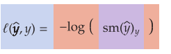
The essence is to first convert some set ofC scores (the values can be any number) into C probabilities (values must be between 0 and 1), and then calculate a loss based on the probability of the true class y. (View Highlight)
Note: Cross-entropy loss
soft maximum (or softmax) function: it converts everything to a non-negative number and ensures that the values sum up to 1.0. (View Highlight)
The average number of bits needed to encode a message when you think it has a distribution but it actually follows the distribution (aka, how much do you need to repeat yourself because you ( ) don’t speak quite the same dialect as your friend ( )) is equal to how often you expect to see token multiplied by the log of how often you actually see token summed over all possible tokens that you might see (and negated to make the number positive instead of negative). (View Highlight)
. Imagine we are ordering lunch for a group of people, and we expect 70% to eat chicken and 30% to eat turkey (see figure 2.7). That’s the predicted distribution q. In reality, 5% want turkey and 95% want chicken. (View Highlight)
Note: TODO: Work this out myself and put it in Obsidian
It is common jargon to call the value that goes into softmax the logits and the outputs ˆy the probabil- ities. (View Highlight)
, the metrics we care about (e.g., accuracy) may not be the same as the loss we used to train our model (e.g., cross-entropy). There are many ways these may not match perfectly, because a loss function must have the property of being differentiable, and most of the time our true goal does not have this property. So we often have two sets of scores: the metrics by which the developers and humans understand the problem and the loss function that lets the network understand the problem. (View Highlight)
New highlights added May 31, 2024 at 12:24 PM
. We use B to denote the batch size; for most applications, you will find B ∈ [32, 256] is a good choice. (View Highlight)
Columnar data (data that could go in a spreadsheet) should use fully connected layers, because there is no structure to the data and fully connected layers impart no prior beliefs. Audio and images have spatial properties that match how CNNs see the world, so you should almost always use a CNN for those kinds of data. (View Highlight)
New highlights added May 31, 2024 at 1:24 PM
For columnar data, shuffling has no real impact because the data has no special structure. Right: When an image is shuffled, it is no longer recognizable. (View Highlight)
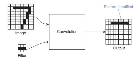
A convolution takes an image and filter and produces one output, the filter defining what kind of “pattern” to look for. The more convolutions you have, the more different patterns you can detect. (View Highlight)
Note: 1D convolution. In 2D, the kernel is a matrix. In 3D, it is a rank-3 tensor; etc.
New highlights added June 2, 2024 at 8:59 AM
Neural networks are really useful and start to out-perform other methods when we use them to impose a prior belief. (View Highlight)
By how we design the network, we impart some knowledge about the intrinsic nature or structure of the data. (View Highlight)
We need to use a transform to convert the images to tensors, which is why we import the transforms package from torchvision. We can simply specify the ToTensor transform, which converts a Python Imaging Library (PIL) image into a PyTorch tensor where the minimum possible value is 0.0 and the max is 1.0, so it’s already in a pretty good numerical range for us to work with. (View Highlight)
In PyTorch, an image is represented as (N, C,W,H),2 but imshow expects a single image as (W,H, C). So we need to permute the dimensions when using imshow (View Highlight)
If we use a convolutional filter of size K, we can use padding of K/2 to make sure our output stays the same size as our input. (View Highlight)
One way we could apply the network fΘ(·) to this larger dataset would be to slide the network across slices of the input and share the weights Θ for each position. (View Highlight)
Note: This discussion is extremely confusing. But the idea is that you have a fully connected linear network that operates on a K-sized region of D, and you use it on eery K-sized subregion of D with the same weights.
Blurring involves taking a local average pixel value and replacing every pixel with the average of its neighbors. This can be useful to wash out small noisy artifacts or soften a sharp edge. (View Highlight)
Designing all the filters you might need by hand was a big part of computer vision for many decades. (View Highlight)
we can let the neural network learn the filters itself. (View Highlight)
each filter looks at all C input channels on its own (View Highlight)
One filter always produces one output chan- nel, regardless of however many input channels there are. (View Highlight)
Because the input has a shape of (C,W), the filter has a shape of (C,K). So when the input has multiple channels, the kernel will have a value for each channel separately. That means for a color image, we could have a filter that looks for “red horizontal lines, blue vertical lines, and no green” all in one operation. But it also means that after applying one filter, we get one output. (View Highlight)
PyTorch provides the nn.Conv1d, nn.Conv2d, and nn.Conv3d functions for handling this for us. Each of these implements a convolutional layer for one-, two-, and three-dimensional data. (View Highlight)
Every output channel is combined into one new image with channels. (View Highlight)
Note: The number of output channels is equal to the number of filters (convolutions) applied.
convolutions impart the prior belief that things located near each other are related, but things far from each other are not related. (View Highlight)
we eventually switch to using a fully connected (View Highlight)
layer, which does not understand the spatial nature of the data. For this reason, the nn.Linear layer learns to look for values (or objects) at very specific locations. (View Highlight)
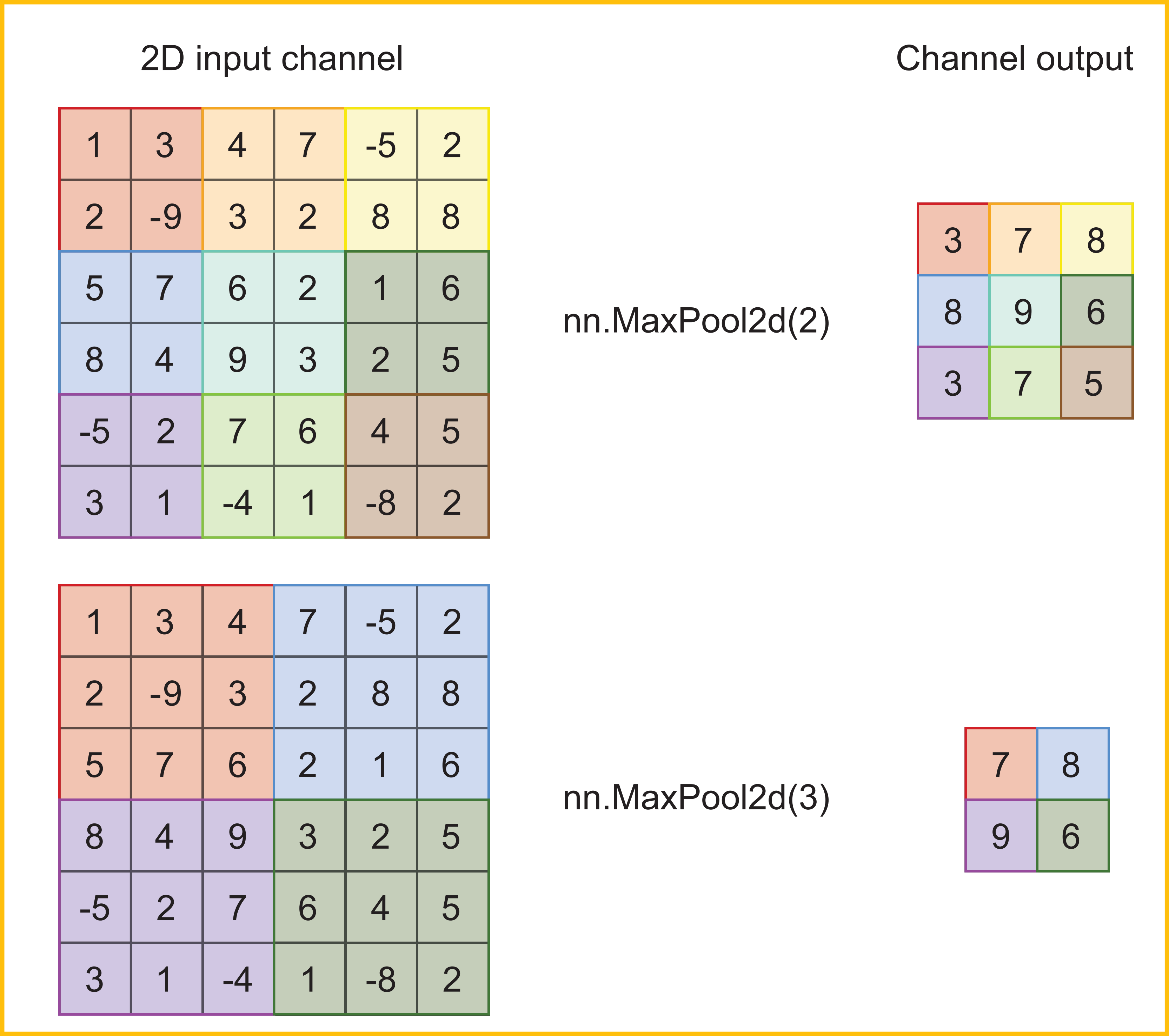
The choice of how many pixels to slide by is called the stride. (View Highlight)
if you use stride=Z for any (positive integer) value of Z, the result will be smaller by a factor ofZ along each dimension (View Highlight)
Having a stride of K means we shrink the size of each shape dimension by a factor ofK. So if our input has a shape of (B, C,W,H), the output of nn.MaxPool2d(K) will be a shape of (B, C,W/K,H/K). (View Highlight)
common practice is to increase the number of filters by K× after every round of pooling so that the total computation done at every layer remains roughly the same (View Highlight)
For real use, you probably want to pick a value of p=0.5 or p=0.15. (View Highlight)
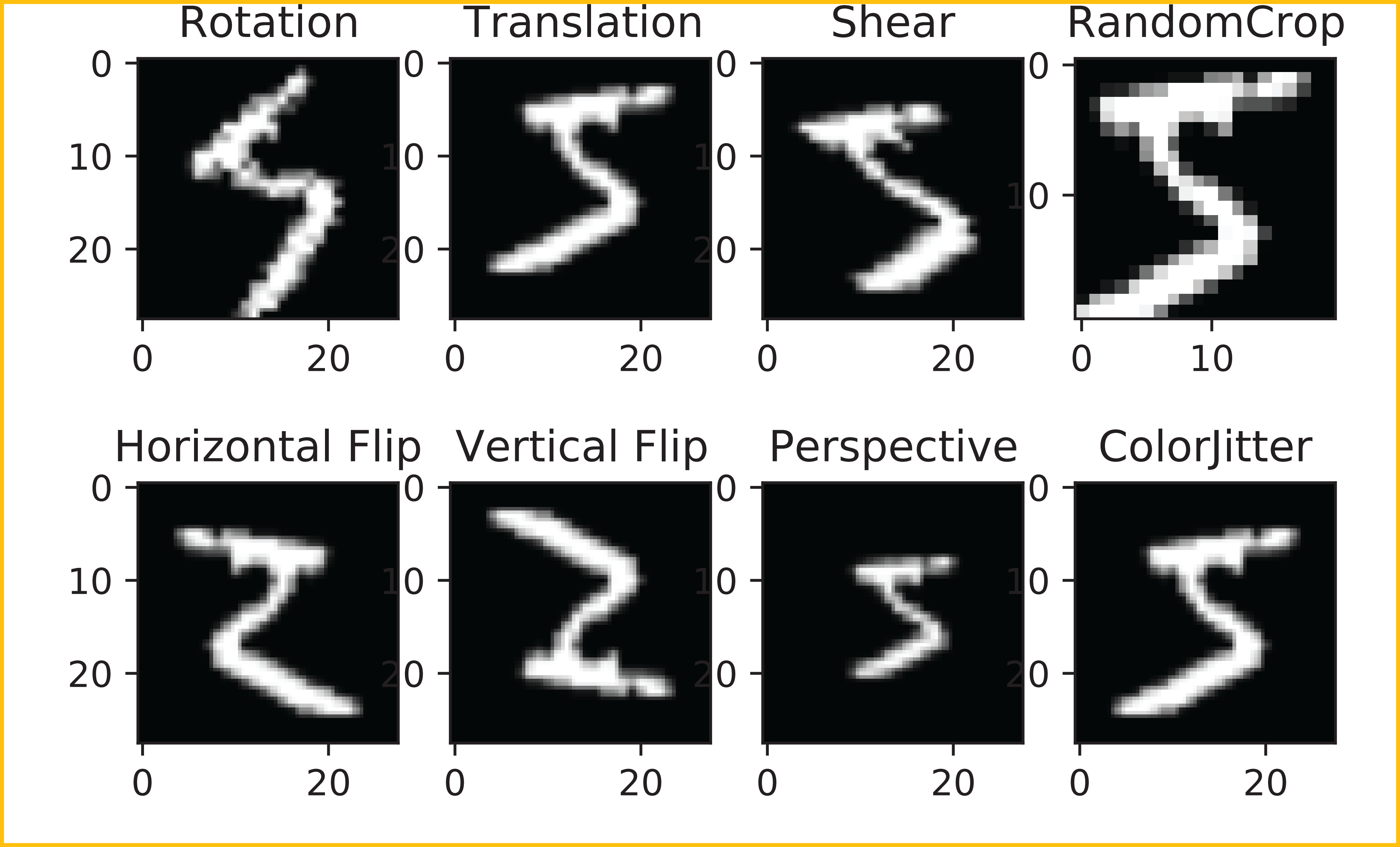
Your best bet for selecting a good set of transforms is to apply them to data and look at the results yourself; if you can’t tell what the correct answer is anymore, chances are your CNN can’t either. (View Highlight)
Because PyTorch uses PIL images as its foundation, you can also write custom transforms to add into the pipeline. This is where you can import tools like scikit-image that provide more advanced computer vision transforms that you can apply. (View Highlight)
Data augmentation also increases the value of training for more epochs. Without augmentation, each epoch revisits the exact same data; with augmentation, your model sees a different variant of the data that helps it better generalize to new data. (View Highlight)
. The RNN takes in a single representation of all previous content ht−1 and information about the newest item in the sequence xt. The RNN merges these into a new representation of everything seen so far ht, and the process repeats until we reach the end of the sequence. (View Highlight)
You may also hear weight sharing called tied weights. (View Highlight)
Some people prefer this terminology if the weights are used slightly differently. (View Highlight)
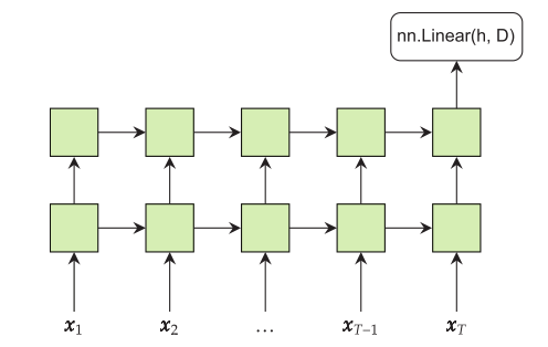
The goal of an RNN is to summarize every item in a sequence of items, using just a single item. (View Highlight)
RNN takes in two items: a tensor ht−1 that represents everything seen so far in the order it has seen, and a tensor xt that represents the newest/next item in the sequence. (View Highlight)
If we have a network module A, where A(x) = h, we can use weight sharing to apply the network module A to every item independently. So, we get T outputs, hi = A(xi) (View Highlight)
one simple improvement is to use stratified sampling to create the train/test split. It’s a common tool and available in scikit-learn (http://mng.bz/v4VM). The idea is that you want to force the sampling to maintain the class ratios in the splits. (View Highlight)
Note: stratified sampling for class imbalance
The RNN classes in PyTorch apply nonlinear activation functions on their own. (View Highlight)
you should not apply a nonlinear activation function afterward, because it has already been done for you. (View Highlight)
Note: This is quite arcane. I have to imagine there is a better way by now.
When working with RNNs, we often have a lot of complex tensor shapes occurring at once. For this reason, I always include a comment on each line indicating how the tensor shapes are changing due to each operation. (View Highlight)
we can again use the train_simple_network function to train our first RNN (View Highlight)
Tensors need all dimensions to be consistent and the same, but our time dimension (in this case, how many characters long each name is) is not consistent. (View Highlight)
This is an abstraction problem because fundamentally, nothing prevents an RNN from working with inputs of varying lengths of time. To fix this, PyTorch provides the packed sequence abstraction (http://mng.bz/4KYV). All types of RNNs available in PyTorch support working on this class. (View Highlight)
PyTorch organizes them by length and begins by in- cluding the first time step of all sequences in one batch over time. As time progresses, the shorter sequences reach their end, and the batch size is reduced to the number of sequences that have not reached their end. (View Highlight)
Packing actually involves two steps: padding (make everything the same length) and packing (store information about how much padding was used). To implement both padding and packing, we need to override the collate function used by the DataLoader. (View Highlight)
Note: This appears to be a kludge due to an oversight in PyTorch, and it’s possible that it’s already fixed by the time I’m reading this.
It turns out the nn.Embedding layer from PyTorch does not handle packed inputs. I find it’s easiest to create a new wrapper Module that takes an nn.Embedding object in the constructor and fixes it to handle packed inputs. (View Highlight)
Note: I don’t understand this. This seems like it would be doing the initial packing, but the fact that input is a PackedSequence suggests it’s already been done.
We put in a lot of extra effort to get the code to work with batches of data, and much of the code online has not bothered to do so. When you learn about a new technique for training or using RNNs, it may not support packed inputs (View Highlight)
Like other approaches we have learned about, you can stack multiple layers of RNNs. However, due to the computational complexity of training RNNs, PyTorch provides highly optimized versions. Rather than manually insert multiple nn.RNN() calls in a sequence, you can pass in an option telling PyTorch how many layers to use. (View Highlight)
My recom- mendation is to look at using two or three layers of the recurrent components in your architecture. (View Highlight)
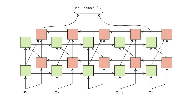
To make it easier for the RNN to get the information it needs from long sequences, we can have the RNN traverse the input in both directions at once and share this information with the next layer of the RNN. (View Highlight)
Notice that the last time step now comes partially from the leftmost and rightmost items in the sequence. (View Highlight)
New highlights added June 3, 2024 at 5:27 PM
Not all local minima are “bad”; if a minimum is sufficiently close to the global minimum, we will probably get good results. (View Highlight)
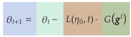
. All of the information and learning come from gt; it controls what the network learns and how well it learns. The learning rate η simply controls how quickly we follow that information. But the gradient gt is only as good as the data we use to train the model. If our data is noisy (and it almost always is), our gradients will also be noisy. (View Highlight)
the exponential learning rate schedule helps solve the problem of getting near the solution but not quite making it to the solution. (View Highlight)
The trick to using the exponential learning rate well is setting ηmin. I usually recommend making it 10 to 100 times smaller than η0. (View Highlight)
Instead of constantly adjusting the learning rate ever so slightly, we let it stay fixed for a while and then drop it dramatically just a few times. (View Highlight)
we go maximum speed for as long as possible but eventually slow down to converge on the solution. (View Highlight)
cosine annealing decreases and increases the learning rate. This approach is very effective for getting the best possible results but does not provide the same degree of stabilization, so it might not work on poorly behaved datasets and networks. (View Highlight)
gradient descent likes to find wide basins as good solutions, and it would be difficult for the optimization to bounce out because the solution is wide. This gives us a little more confidence that this crazy cosine schedule is a good idea, and empirically it has performed well on a number of tasks (image classification, natural language processing, and many more). In fact, cosine annealing has been so successful that there have been dozens of proposed alternatives. (View Highlight)
None of them use information about how well the learning is going. (View Highlight)
The primary information we have is the loss for each epoch of training, and we can add it into our approach to try to maximize the accuracy of our final model. This is what the plateau-based strategy does, and it will often get you the best possible accuracy for your final model. (View Highlight)
If the test loss has stabilized, that would be a good time to reduce the learning rate.2 (View Highlight)
This is the idea behind the reduce learning rate on plateau schedule, implemented by the ReduceLROnPlateau class in PyTorch. (View Highlight)
ReduceLROnPlateau has three primary arguments to control how well it works. First is patience, which tells us how many epochs of no improvement we want to see before reducing the learning rate. (View Highlight)
The second argument is threshold, which defines what counts as not improving. (View Highlight)
The last parameter is the factor by which we want to drop the learning rate η every time we determine that we have hit a plateau. (View Highlight)
you can’t use the test data to choose when to alter the learning rate. Doing so will cause overfitting because you are using information about the test data to make decisions and then using the test data to evaluate your results. Instead, you need to have training, validation, and testing splits. (View Highlight)
Note: Breaks a batch of data into a tuple of two batches, with the composition of each set being random
There are two particular cases where Reduce (View Highlight)
First is the case where you don’t have much data. T (View Highlight)
The second case is when your data strongly violates the identically and independently distributed (IID) assumption. (View Highlight)
we would like to have a global learning rate η and individualized learning rates ηj for all of the parameters. While the global learning rate stays fixed (unless we use a learning rate schedule), we let some algorithms adjust each of the ηj values to try to improve convergence. (View Highlight)
notice that the exponents above µ get larger every time we apply another round of momentum. This makes the contributions of very old gradients become essentially zero as we keep updating. (View Highlight)
If you want to get the best possible accuracy from your network, SGD with some form of momentum is still considered one of the best options. The downside is that finding the combination of µ and η values that gives the absolute best results is not easy and requires training many models. (View Highlight)
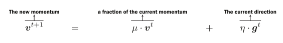
Calculate a provisional set of updated parameters based only on momentum.
Calculate a provisional gradient based on a the mini-batch and the provisional gradient. Use this to compute a velocity.
The new parameters are the old parameters minus the velocity from step 2.
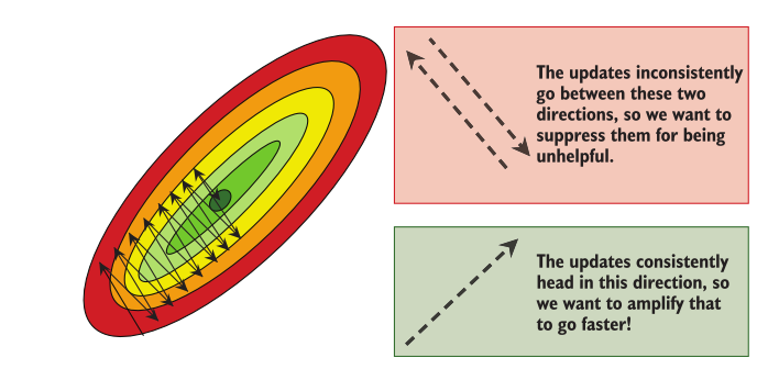
Now, think about this scenario under Nesterov momentum. We are at the solution, and first we follow the velocity, pushing us away from the goal. Then we calculate the gradient, which recognizes that we need to head back in the opposite direction and thus move toward the goal. When we add these two together, they almost cancel out (we take a smaller step forward or backward, depending on which has a larger magnitude, gt or vt). In one step, we have started to change the direction in which our optimizer is headed, whereas normal momentum would take two steps. (View Highlight)
Note: “This scenario” refers to the situation where we have reached a minimum, but we don’t know it.
you won’t usually see one version of momentum perform dramatically better or worse than the other. (View Highlight)
Adam is my current favorite approach because it has default parameters that just work, so I don’t have to spend time tuning them. (View Highlight)
New highlights added June 4, 2024 at 9:15 AM
If one parameter gt j has high variance, we probably don’t want to let it contribute too much to the momentum (View Highlight)
because it will likely change again. If a parameter gt j has low variance, it’s a reliable direction to head in, so we should give it more weight in the momentum calculation. (View Highlight)
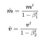
Note: Adam involves estimating the recent mean and variance of each term in the gradient. Because the mean and variance are initialized to zero, we also apply an adjustment. The resulting vector is multiplied by the learning rate to obtain the change in the parameter vector.
The numerator η· ˆm is computing the SGD with momentum term, but now we are normalizing each dimension by the variance. That way, if a parameter has naturally large swings in its value, we won’t adjust as quickly to a new large swing— because it usually is quite noisy. If a parameter usually has a small variance and is very consistent, we adapt quickly to any observed change. The term is a very small value so we never end up dividing by zero. (View Highlight)
Note: Chaudhary had a nice analogy: if someone talks all the time, I don’t pay a great deal of attention to any particular thing they say; but if they rarely speak, and they decide to now, that’s worth taking note of.
The original paper for the Adam algorithm contained a mistake, but the proposed algorithm still worked well for the vast majority of problems. A version that fixes this mistake is called AdamW and is the default we use in this book. (View Highlight)
if any (absolute) value in a gradient is larger than some threshold z, just set it to a maximum value of z (View Highlight)
Note: gradient clipping
The idea is that any value larger than our threshold z clearly indicates the direction; but it is set to an unreasonable distance, so we forcibly clip it to something reasonable. (View Highlight)
If I’m working with recurrent neural networks, I always use gradient clipping because the recurrent connections tend to cause exploding gradients, making them a common issue in that scenario (View Highlight)
grid search works well only for optimizing one or (View Highlight)
two variables at a time due to its exponential cost as more variables are added. (View Highlight)
Unlike grid search, it requires fewer decisions, finds better parameter values, can handle more hyperparameters, and can be adapted to your computational budget (i.e., how long you are willing to wait). (View Highlight)
Note: Optuna
Optuna can be used with any framework, as long as you can describe the goal as a single numeric value. (View Highlight)
Optuna does a better job of hyperparameter optimization by using a Bayesian technique to model the hyperparameter problem as its own machine learning task. (View Highlight)
Optuna quickly figures out that there is no way to find a better solution in these parts of the space and stops exploring those areas. This allows it to spend more time looking for the best solution and to better handle more than just two parameters. (View Highlight)
we have to create new training and validation splits using only the original training data. Why? Because we will reuse the validation set multiple times, and we do not want to overfit to the specifics of our validation data. (View Highlight)
Note: I assume they mean we need to do this for each iteration?
Note: Why 4 here? Remind myself based on CNN chapter
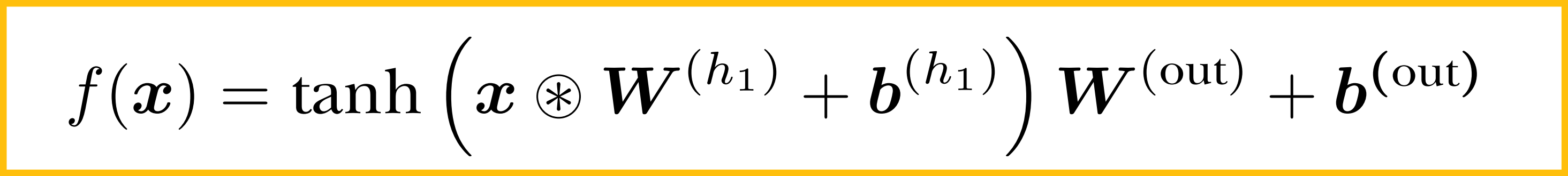
Both tanh(·) and σ(·) can lead to a problem called vanishing gradients. (View Highlight)
For both tanh(·) and σ(·), if the input x keeps getting larger, both activations saturate at the value 1.0. (View Highlight)
Note: Saturating functions lead to vanishing gradients
there are some cases where you want saturation (we’ll see an example at the end of this chapter with the LSTM) (View Highlight)
Saturating activations are not the only cause of vanishing gradients. (View Highlight)
If you are using an activation function that can saturate, you can also plot a histogram of the activation functions to check whether that is the cause of vanishing gradients (View Highlight)
For most use cases, simply replacing tanh(·) or σ(·) with the ReLU activation will allow your model to converge to a more accurate solution in fewer epochs. However, the ReLU often performs worse for very small networks. (View Highlight)
Instead of having a vanishing gradient, the ReLU has no gradient for x ⇐ 0. If you have a lot of neurons, it is OK if some of them “die” and stop activating; but if you don’t have enough extra neurons, it becomes a serious problem. (View Highlight)
leaky ReLU takes a “leaking” factor α, which is supposed to be small. Values in the range α ∈ [0.01, 0.3] are often used, and the specific value has relatively little impact in most cases. (View Highlight)
PReLU, which attempts to learn what α should be for the LeakyReLU, removing it as a hyperparameter (View Highlight)
There are also “smooth” extensions to the ReLU like CELU, GELU, and ELU, which have been derived to have certain properties. (View Highlight)
you’ll generally be safe and in good company using any ReLU variants as your default choice (View Highlight)
Before we train our neural networks, we again usually do normalization or standardiza- tion before passing the data into the first layer of our network. (View Highlight)
Normalization layers are applied at every layer with one extra trick: let’s let the network learn how to scale the data instead of assuming that a mean of 0 and standard deviation of 1 are the best choices. (View Highlight)
Note: Normalization layers are affine transformations introducing two parameters each: a scaling factor and an offset .
This means µ, σ, γ, and β have a shape of (D), and each item in the batch is normalized by the mean and standard deviation ofjust that batch ofdata. (View Highlight)
Note: Turns out Python 3 lets you use a subset of the Unicode alphabet (including Greek letters) as identifier names, but discourages it
Because it averages over the batch dimension of the tensor, BN is sensitive to the batch size during training and is impossible to use with a batch size of 1. (View Highlight)
What if we have one-dimensional data of shape (B, C,D)? In this case, we normalize the channels over the batch. This means µ, σ, γ, and β each have a shape of (C). (View Highlight)
Note: This is a little unclear; consult documentation for torch.nn.BatchNormd
Why does LN take a list of integers? This list tells LN, from right to left, which values to average over. So if we have a 2D problem with tensors of shape (B, C,W,H), we give LN the last three dimensions as a list [C, W, H]. That covers all the features, which is what we want LN to normalize over. This makes LN a little trickier for CNNs because we also need to pay attention to how large the width and height are, and they change every time we apply max pooling. (View Highlight)
BN is really only useful for fully connected layers and convolutional models, so PyTorch can easily hardcode it to the two tasks. LN can be helpful for almost any architecture (e.g., RNNs), and the list of integers telling LN explicitly what to normalize over allows us to use the same Module for these varieties of use cases. (View Highlight)
For non-recurrent networks, using BN is a good idea provided you can train on batches B ≥ 64. If your batch isn’t big enough, you won’t get a good estimate of µ and σ, and your results could suffer. (View Highlight)
LN should be your first pick whenever you reuse a subnetwork with weight sharing: BN’s statistics assume one distribution, and when you do weight sharing, you get multiple distributions, which can cause problems. (View Highlight)
Note: Also helpful when you have to use smaller batches
our optimization approach is not perfect, so it is always the case that what a model can learn must be less than or equal to what it can represent. (View Highlight)
Normalization layers are unique in that they do not increase capacity. Said another way, their representational capacity does not change, but what they can learn improves. (View Highlight)
Normalization is a linear operation, and any consecutive sequence of linear operations is equivalent to one linear operation (View Highlight)
Note: Therefore normalization does not add representational capacity
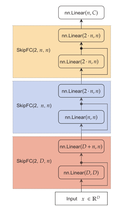
skip connections can shrink the gap between a network’s capacity (what it could represent) and what it can learn (what it learns to represent) (View Highlight)
having every layer connect directly to the output can be overkill and eventually make the learning problem more difficult. Imagine if you had 100 hidden layers, all connected directly to the output layer—that would be a huge input for the output layer to deal with (View Highlight)
this approach has been used successfully8 by organizing “blocks” of dense skip connections. (View Highlight)
Note: How did he choose the dimensionality of each of these blocks?
encap- sulating the non-feed-forward parts into a custom Module is my preferred approach to organize custom networks: (View Highlight)
skip connections were more effective on their own before normalization layers were invented to help tackle the same problem (View Highlight)
New highlights added June 4, 2024 at 12:14 PM
we can’t do skips across the MaxPool2d layer. Pooling changes the width and height of the image, and we would get an error if we tried to concatenate two tensors of shape (B, C,W,H) and (B, C,W/2,H/2) (View Highlight)
skip connections form one of the basic building blocks of a more powerful and routinely successful technique called a residual layer that is reliably more effective. (View Highlight)
a convolution with k = 1 is looking not at spatial neighbors but at spatial channels by grabbing a stack ofCin values and processing them all at once (View Highlight)
Note: 1x1 convolutions still convert from to channels, which makes them useful when channel depth is an issue
In essence, we are giving the network a new prior: that it should try to share infor- mation across channels, rather than looking at neighboring locations. (View Highlight)
we are telling the network to focus on the patterns found at this location instead of having it try to build new spatial patterns (View Highlight)
if we combine skip connections and 1 × 1 convolutions in just the right way, we get an approach called a residual con- nection that converges faster to more accurate solutions (View Highlight)
The block is a kind of skip connection where two layers combine at the end, creating long and short paths. (View Highlight)
Note: When using residual blocks with convolutions, apply a 1x1 convolution to the short path to match the short path’s dimensionality to that of the long path
the second 1×1 expands the result back up (View Highlight)
Note: Here we are actually using the 1x1 convolution to add channels back, i.e., to map from a lower- to a higher-dimensional space.
An entire area of machine learning studies compression as a tool to make models learn interesting things. (View Highlight)
it is hard to overstate how large an impact residual connections have had on modern deep learning, and you should almost always default to implementing a residual-style network (View Highlight)
In many cases, using ResNet with no change except to the output layer gives a strong result on an image classification problem (View Highlight)
One of the challenges with learning an RNN is that, when unrolled through time, many operations are performed on the same tensor. It is hard for the RNN to learn how to use this finite space to extract information it needs from the fixed-sized representation of a variable number of timesteps, and then to also add information to that representation. (View Highlight)
it’s easy for the gradient to send information back when there are fewer operations on it. If we have a sequence with 50 steps, that’s like trying to learn a network with 50 layers with 50 more opportunities for gradient noise to get in the way. (View Highlight)
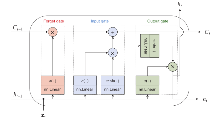
the LSTM creates two sets of states: a hidden state ht and a context state Ct (View Highlight)
ht does the work and tries to learn complex functions, and the context Ct tries to simply hold valuable information for use later. (View Highlight)
Note: An LSTM adds gate parameters that determine:
(i) how much information to remove from the long-term context vector;
(ii) how much information to add to the long-term context vector; and
(iii) how much information from the long-term context vector to incorporate into the short-term hidden state.
The context Ct acts kind of like a short path: few (and simple) operations are performed on it, making it easier for the gradient to flow back over very long sequences. (View Highlight)
The GRU has the same inspiration as the LSTM but tries to get the hidden state ht to do double-duty as the short- and long-term memory. This makes the GRU faster, use less memory, and is easier to write code with, which is why we use it. The downside is that the GRU is not always as accurate as the LSTM. By contrast, the LSTM with peephole connections has been a tried-and-true method that is hard to beat and is what people are usually referring to when they say an “LSTM.” (View Highlight)
The LSTM is one of the few tried-and-true deep learning methods that has lasted for decades without much change. If you need an RNN, the LSTM is a good default choice. The gated recurrent unit (GRU) we mentioned is also a good choice, particularly if you need something that requires less computational resources. (View Highlight)
New highlights added June 5, 2024 at 10:55 AM
The idea behind self-supervision is that we use a regression or classification loss function to do the learning, and we predict something about the input data x itself. (View Highlight)
coming up with new approaches all the time. (View Highlight)
bread-and- butter principal component analysis (PCA) works by secretly being an autoencoder. (View Highlight)
Note: Hi Dr. Raff,
I enjoyed reading Inside Deep Learning. I’m not sure, however, about the claim that “principal component analysis (PCA) works by secretly being an autoencoder” (p. 255).
PCA is characterized by its mechanism, which is based on finding the eigenvalues of a covariance matrix of a higher-dimensional sample/population space, and then projecting vectors into a subspace spanned by the eigenvectors corresponding to the largest eigenvalues (the ‘principal components’ of the matrix).
PCA can be approximated by a neural network because the Universal Approximation Theorem (Cybenko Theorem) states that any function can be approximated to arbitrary precision by some feed-forward neural network with at least one hidden layer. But the network is not actually performing this function.
This seems to me to be an important distinction, especially in the era of LLMs. An LLM can simulate human speech with chilling precision. But (thank goodness) they do not do so for the same reasons.
Likewise, the learned weights of a neural network may produce output that is arbitrarily similar to an orthogonal projection onto the principal axes of a higher-dimensional space. The weight matrix of the final layer may even be arbitrarily close to the corresponding projection matrix (though I don’t think they need to?). I still don’t think that’s PCA.
This is not to detract from the utility of this book, which I greatly appreciate. Thank you for writing it.
Best wishes,
David Borenstein
. Autoencoding means we generally learn two functions/networks: first a function fin(x) = z, which transforms the input x into a new representation z ∈ RD , and then a function fout(z) = x, which converts the new representation z back into the original representation. (View Highlight)
This assumes that there is a representation z to be found that somehow captures information about the data x but is unspecified. We don’t know what z should look like because we have never observed it. For this reason, we call it a latent representation of the data because it is not visible to us but emerges from training the model. (View Highlight)
We have one weight matrix W acting as the encoder, and its transpose W is acting as the decoder. That means PCA is using weight sharing (remember that concept from chapters 3 and 4?). (View Highlight)
Note: In working through his “proof” of this, the author claims that is explicitly a form of weight sharing across two layers, one with weights and the other with weights . He then codes up a TransposeLinear PyTorch module that he adds to the network. Its forward method is return F.linear(x, self.weight.t(), self.bias).
The author has thus forced the network to have an architecture similar to PCA. This injects a strong prior belief that the optimal solution looks like an orthogonal projection. Claiming that this proves PCA is an autoencoder is a circular, and ultimately fatuous, argument.
Autoencoding networks are also useful for outlier detection. (View Highlight)
what if we made the target size larger than the original input? (View Highlight)
. If we let the encoding dimension become too large, it may be good at performing reconstructions on easy data, but it is not robust to changes and noise. (View Highlight)
A denoising autoencoder adds noise to the encoder’s input while still expecting the decoder to produce a clean image. (View Highlight)
Ifyou can make synthetic noise that is realistic to the issues you might see in real life, you can create models that remove the noise and improve the accuracy by making the data cleaner. (View Highlight)
Note: I believe this doesn’t apply at inference time, but it would be nice to know for sure
Dropout still works as a regularizer and is useful and used, but it is not ubiquitous as it once was. The tools we have learned thus far, like normalization layers, better optimizers, and residual connections, give us most of the benefits of dropout. (View Highlight)
dropout is applied differently at training versus test time. (View Highlight)
Let’s say you have t steps of your data: x1, x2, … , xt−1, xt. The goal ofan autoregres- sive model is to predict xt+1 given all the previous items in the sequence. The mathy way to write this would be P(xt+1|x1, x2, … , xt) (View Highlight)
The autoregressive approach is still a form of self-supervision because the next item in a sequence is a trivial component of having the data in the first place. (View Highlight)
at step , the input from the next step is used as the label for computing a loss. (View Highlight)
Note: autoregressive model
While RNNs are an appropriate and common architecture to use for auto- regressive models, bidirectional RNNs are not. (View Highlight)
If we used a bidirectional model, we would have information about the future content in the sequence (View Highlight)
Grabs the label substring by shifting over by 1 (View Highlight)
Note: The label for an autoregressive dataset is another substring of the same length as the input, offset by 1
Note: This block is quite confusing, because the author buried the key operation, self.step(x_in, h_prevs), inside the append. But the idea is that, at each time step:
We obtain the next embedding.
We calculate the next hidden state based on the obtained embedding and all of the preceding hidden states.
We append the new hidden state to the history of hidden states.
. First we check the shape of the input, and if it has only one dimension, we assume that we need to embed the token values to make vectors (View Highlight)
Note: Why wouldn’t we just make sure we already did this? Seems like a bad design.
These are both good defensive code steps to make sure our function can be versatile and avoid errors (View Highlight)
Note: NO, THEY’RE NOT! They secretly perform coercions and force step to know about things outside of its responsibilities. These are great ways to introduce bugs. Jesus.
Note: pred_class is a small FC network that projects the hidden state back into the vocabulary size. What’s missing here, compared with most applications of autoregressors for text, is a sampling step based on the softmax of the resulting logits that chooses a next token (which in this example is a character, not a word).
PyTorch has a simple trick that nn.Linear layers are applied to the last axis of a tensor regardless of the number of axes. (View Highlight)
Autoregressive models are not only self-supervised; they also fall into a class known as generative models. This means they can generate new data that looks like the original data it was trained on. (View Highlight)
The temperature is a scalar that we divide the model’s prediction by before computing the softmax to make probabilities (View Highlight)
Something with infinite temperature will result in uniformly random behavior (not what we want), and something with zero temperature is frozen solid and returns the same (most likely) thing over and over again (also not what we want) (View Highlight)
Adjusting the temperature is but one of many possible techniques for selecting the generated output in a more realistic-looking manner. Each has pros and cons, but you should be aware of three alternatives: beam search, top-k sampling, and nucleus sampling (View Highlight)
Note: I am not annotating this chapter, because I believe that the author does not fully understand attention.
My understanding of attention is that it is an explicit mechanism to establish a correspondence between a key and a query. IIRC, it was introduced in Bahdanau, et al. as a way to facilitate alignment of input and output sequences in an encoder-decoder network for machine translation. Without the context vector, the decoder had only the final hidden state to work with. Attention, in the form of a context vector, allowed the model to attend to each hidden state (corresponding to an input token) during decoding.
The author claims that an attention mechanism is anything that causes a model to ignore “less relevant” input. As a toy example, the author whose input is a bag of images from MNIST. The output is the highest observed numeric value in the bag. To accomplish this, the author adds a softmax after predicting the label for each input. This downweights lower values, causing the model to “attend to” the highest one. Thus, the author claims, the model uses attention.
This seems like a stretch. The softmax is encoding a prior belief that higher values are more likely to contain the correct label. This is a good idea, and is a nice way to solve the problem. However, if encoding a prior belief about the relative importance of information constitutes “attention,” then convolutions (which “attend to” shapes) are also attention. Clearly they are not.
Note: It appears that, at least according to the author, an “attention” mechanism is anything that causes a model to ignore less-important data based on context.
In the book’s toy example, we are training a model to label the image corresponding to the highest observed value in a bag of MNIST images. By softmaxing the predicted class of each image, we overweight the largest one.
This is a good idea, but I don’t really think it qualifies as “attention”: it’s encoding a prior that higher values are more likely to be the right class, but it wouldn’t tune out, say, a garbled image.
 (View Highlight)
 (View Highlight)
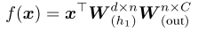 (View Highlight)
 (View Highlight)
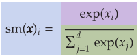 (View Highlight)
 (View Highlight)
 (View Highlight)
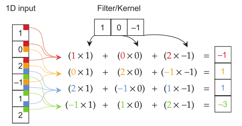 (View Highlight)
 (View Highlight)
 (View Highlight)
 (View Highlight)
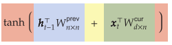 (View Highlight)
 (View Highlight)
 (View Highlight)
 ?t=1717347651271 (View Highlight)
 (View Highlight)
 (View Highlight)
 (View Highlight)
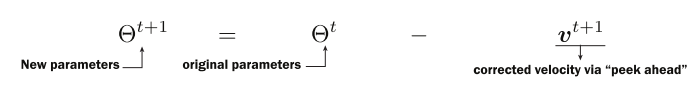 (View Highlight)
 (View Highlight)
 (View Highlight)
 ?t=1717515509268 (View Highlight)