Chaudhury 2024, ch. 4 (linear algebraic tools for ML)

Notes from Chaudhury, et al. (2024), chapter 4

Highlights

• Given a square symmetric matrix A, the scalar quantity Q = xTAx is called a quadratic form. (View Highlight)
•  x− 훼 T I x− 훼 = r2   (View Highlight)
• The original x0, x1-based equation only works for two dimensions. The matrix based equation is dimension agnostic: it represents a hypersphere in an arbitrary-dimensional space. For a two- dimensional space, the two equations become identical. (View Highlight)

New highlights added June 19, 2024 at 5:30 PM

• Quadratic forms are also found in the second term of the multidimensional Taylor expansion (View Highlight)
• Another huge application of quadratic forms is PCA (View Highlight)
• because the quadratic form is part of the multidimensional Taylor series, we need to minimize quadratic forms when we want to determine the best direction to move in to minimize the loss L  x . (View Highlight)
• we discuss quadratic forms with unit vectorsQ = ˆxTAˆ (View Highlight)
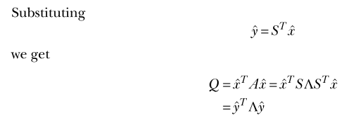• (View Highlight)
• ?t=1718831035175 (View Highlight)
  • Note: Why y-hat squared is a unit vector. I have a note in Obsidian about why you can do this trick with the product of the transpose matrix.
• (View Highlight)
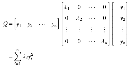
  • Note: I have a note in Obsidian about why you can get this nice sum out of this quadratic form.
• The quantity n i=1 휆i y2 i , where n i=1 y2 i =1 and 휆1 ≥ 휆2 ≥ · · · 휆n, attains its maximum value when y1 =1, y2 = · · · yn = 0. (View Highlight)
  • Note: To be clear, they are saying
• the quadratic form Q = ˆxTAˆx attains its maximum when ˆx is along the eigen- vector corresponding to the largest eigenvalue of A. The corresponding maximum Q is equal to the largest eigenvalue of A. Similarly, the minimum of the quadratic form occurs when ˆx is along the eigenvector corresponding to the smallest eigenvalue. (View Highlight)

New highlights added June 21, 2024 at 11:08 AM

• The matrix A amplifies the vector x to b= Ax. So we can take the maximum possible value of Ax over all possible x; that is a measure for the magnitude of A. (View Highlight)
• the spectral norm is given by the largest eigenvalue of ATA A2 =max Aˆx = 휎1 (View Highlight)
  • Note: Notes should recapitulate the derivation of the spectral norm
• it is the root mean square of all the matrix elements (View Highlight)
  • Note: WRONG — it is proportional to the RMS, but it lacks a normalization by , so it is not actually RMS.
• singular values (eigenvalues of ATA) (View Highlight)
  • Note: Note that “singular” here has absolutely nothing to do with the non-invertibility. Rather, the etymology of both comes from an idea of specialness.
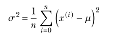• (View Highlight)
  • Note: Variance is the average distance of each value from the mean. Covariance generalizes this idea to higher dimensions.
• manning.book (View Highlight)
• (View Highlight)
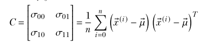
  • Note: Covariance matrix. Note that the sum on the right is an outer product, not a dot product.
• the component of any vector along a direction is yielded by the dot product of the vector with the unit direction vector (View Highlight)
• C =ˆlTCˆl is the variance of the data components along the direction ˆl. As  such, it represents the spread of the data along that direction. What is the direction ˆl along which this spread ˆlTCˆlis maximal? It is the direction ˆlthat maximizes C  =ˆlTCˆl. This maximizing direction can be identified using the quadratic form optimization technique (View Highlight)
• Variance is maximal when ˆlis along the eigenvector corresponding to the largest eigenvalue of the covariance matrix C (View Highlight)
• PCA assumes that the underlying pattern is linear in nature. Where this is not true, PCA will not capture the correct underlying pattern. (View Highlight)
• There are several slightly different forms of SVD. (View Highlight)
• The SVD theorem states that any matrix A, singular or nonsingular, rectangular or square, can be decomposed as the product of three matrices A=UΣVT (4.11) where (assuming that the matrix A is m× n) Σ is an m× n diagonal matrix. Its diagonal elements contain the square roots of the eigenvalues of ATA. These are also known as the singular values of A. The singular values appear in decreasing order in the diagonal of Σ. V is an n × n orthogonal matrix containing eigenvectors of ATA in its columns. U is an m×m orthogonal matrix containing eigenvectors of AAT in its columns. (View Highlight)