(La Rocca) Advanced Algorithms and Data Structures

Advanced Algorithms and Data Structures

Metadata

• Author: Marcello La Rocca
• Full Title: Advanced Algorithms and Data Structures
• Category:books
• Summary: The text discusses advanced algorithms and data structures like heaps, priority queues, and binary trees for efficient operations like finding nearest neighbors and range queries in datasets. The importance of balanced trees and careful handling of data structures to ensure fast search operations is highlighted. Various algorithms and methods are presented, with examples and references for further exploration provided throughout the text.

Highlights

• the size of the static array in the upper half is constant (it always has three elements), while the dynamic array in the other half starts with size 2, its size is only increased (doubled, actually) when an element is added to a full array. (View Highlight)
• Elements in arrays must all have the same type and require the same space to be stored. (View Highlight)
• Because they are allocated in a single block of memory, arrays are more likely to show the so-called locality of reference (View Highlight)
• every position in an array can be accessed in constant time (View Highlight)
• While random access is one of the strengths of arrays, other operations are slower for them. (View Highlight)
• The empty list is assumed as a primitive, a building block, and each non-empty list is recursively defined as its first element followed by its tail, a shorter, possibly empty list of the remaining elements. (View Highlight)
  • Note: Linked list
• we only need to update the head reference with a new node and update the links for this new node and the old head (unless the list was empty). (View Highlight)
  • Note: Inserting into a singly linked list from the beginning
• At the end—This is not a very practical solution, because we would need to traverse the whole list to find the last node (View Highlight)
• We could think about keeping an extra pointer for the tail of the list, but this would cause an overhead (View Highlight)

New highlights added May 27, 2024 at 2:06 PM

• In any other position—This is useful when keeping the list ordered. However, it’s also expensive, requiring linear time in the worst case, as shown in figure C.8. (View Highlight)
  • Note: Except you can keep an outside pointer if you know you need to insert before/after a specific node that you’re tracking
• They can indeed be seen as a generalization of linked lists (View Highlight)
  • Note: Trees are generalizations of linked lists
• A binary tree is a tree where the number of children for any node is at most 2, meaning that each node can have either 0, 1, or 2 children. (View Highlight)
• A binary search tree (BST) is a binary tree where each node has a key associated with it, and satisfies two conditions: if key(x) is the key associated with a node x, then • key(x) > key(y) for every node y in the left subtree of x. • key(x) < key(z) for every node z in the right subtree of x. (View Highlight)
• • A balanced tree is a tree where for each node, the height of its left and right subtrees differs at most by 1, and both its left and right subtrees are balanced. • A tree is a complete tree if it has height H and every leaf node is either at level H or H-1. • A perfectly balanced tree is a balanced tree in which, for each internal node, the heights of its left and right subtrees are the same. • A perfectly balanced tree is also complete*.* (View Highlight)
• For a binary tree with n nodes, log(n) is the shortest possible height. (View Highlight)
• for the same set of elements, their shape and height can vary greatly depending on the sequence of insertions for those elements (View Highlight)
• there are several solutions that allows us to keep BSTs balanced without degrading performance for insert or delete (View Highlight)
• • 2-3 search trees • red-black trees • B-trees • AVL trees (View Highlight)
  • Note: TODO look up each of these variants of BST
• The division method—Given an integer key k, we define its hash h(k) as h(k) = k%M (View Highlight)
  • Note: Simple hashing strategy
• The multiplication method: h(k) = ⎣ M ⋅ (k ⋅ A%1) ⎦ where 0 < A < 1 is a real constant, and (k*A % 1) is the fractional part of k*A. (View Highlight)
  • Note: Simple hashing strategy
• The pigeonhole principle states that if the number of possible key values to store is larger than the available slots, at some point, we are bound to have two different keys mapped to the same slot (View Highlight)
  • Note: This is not as pointless and stupid a “principle” as it initially sounds. For example, to quote Wikipedia:

    The principle can be used to prove that any lossless compression algorithm, provided it makes some inputs smaller (as “compression” suggests), will also make some other inputs larger. Otherwise, the set of all input sequences up to a given length L could be mapped to the (much) smaller set of all sequences of length less than L without collisions (because the compression is lossless), a possibility that the pigeonhole principle excludes.

• There are two main ways to solve conflicts due to different keys mapping to the same slot: • Chaining—Each element in the array stores a link to another data structure, holding all the keys mapped to that element (see figure C.11). (View Highlight)
• Open addressing—We store elements directly in the array, and on conflicts we generate (deterministically) another hash value for the next position to try. (View Highlight)
• Open addressing allows us to save memory, because there are no secondary data structures, but has some problems that make it rarely the best choice. First and foremost, deleting elements becomes too complicated, and because the size of the hash table is limited and decided on creation, this means that these tables will fill up quickly and need to be reallocated. Even worse, elements tend to group in clusters and, when the table gets populated, many attempts are needed to find a free slot—basically there is a high probability that a linear number of attempts will already be needed when the table is nearly half-full. (View Highlight)
• For a hash table using chaining and linked lists, where the table has size m and contains n elements, all operations require on average O(n/m) time. (View Highlight)

Advanced Algorithms and Data Structures

Metadata

• Author: Marcello La Rocca
• Full Title: Advanced Algorithms and Data Structures
• Category:articles
• Summary: The text discusses advanced algorithms and data structures, including k-d trees and SS-trees for similarity search. These structures help efficiently organize and search through data points in multidimensional space. Various helper functions and methods are provided to optimize tree traversal and operations like insertion and nearest neighbor search.
• URL: https://readwise.io/reader/document_raw_content/178048048

Highlights

• A priority queue is an abstract data structure that can be implemented in many ways (including as a sorted list). A heap is a concrete implementation of the priority queue using an array to hold elements and specific algorithms to enforce invariants. (View Highlight)
• For the implementation of a priority queue, we will initially consider three naïve alter- natives using core data structures discussed in appendix C: an unsorted array, where we just add elements to its end; a sorted array, where we make sure the ordering is reinstated every time we add a new element; and balanced trees, of which heaps are a special case. (View Highlight)
• A binary heap is the most used version of priority queues. (View Highlight)
• e in reality an underlying array is used to store heap’s elements, it can concep- tually be represented as a particular kind of binary tree, abiding by three invariants:  Every node has at most two children.  The heap tree is complete and left-adjusted. (View Highlight)
• Every node holds the highest priority in the subtree rooted at that node. (View Highlight)
• Properties (1) and (2) allow for the array representation of the heap. (View Highlight)
• In the array representation, if we are starting to count indices from 0, the children of the i-th node are stored in the positions8 (2 * i) + 1 and 2 * (i + 1), while the parent of node i is at index (i - 1) / 2 (except for the root, which has no parent). (View Highlight)
• there is no reason to keep our branching factor10 fixed and equal to 2. On the contrary, we can use any value greater than 2, and use the same array representation for the heap. (View Highlight)
• For a d-ary heap, where the branching factor is the integer D > 1, our three heap invariants become  Every node has at most D children.  The heap tree is complete, with all the levels that are left-adjusted. That is, the i-th sub-tree has a height at most equal to its siblings on its left (from 0 to i-1, 1 < i ⇐ D).  Every node holds the highest priority in the subtree rooted at that node. (View Highlight)
• for D = 1, the heap becomes a sorted array (or a sorted doubly linked list in its tree representation) (View Highlight)
• When an element has a higher priority than its parent, it is necessary to call the bubbleUp method (View Highlight)
• The pushDown method handles the symmetric case where we need to move an element down toward the leaves of the heap, because it might be larger than (at least) one of its children. (View Highlight)
• function insert(element, priority) p ← Pair(element, priority) pairs.append(p) bubbleUp(pairs, |pairs| – 1) (View Highlight)
• Priority queues are crucial to implementing Dijkstra and A* algorithms (View Highlight)
• When the size of the heap is larger than available cache or than the available mem- ory, or in any case where caching and multiple levels of storage are involved, then on average a binary heap requires more cache misses or page faults than a d-ary heap. Intuitively, this is due to the fact that children are stored in clusters, and that on update or deletion, for every node reached, all its children will have to be examined. The larger the branching factor becomes, the more the heap becomes short and wide, and the more the principle of locality applies. D-way heap appears to be the best traditional data structure for reducing page faults.23 N (View Highlight)
• An associative array (also referred to as dictionary,3 symbol table, or just map), is com- posed of a collection of (key, value) pairs, such that  Each possible key appears at most once in the collection.  Each value can be retrieved directly through the corresponding key. (View Highlight)
• if the domain (the set of possible keys) is small enough, we can still use arrays by defining a total ordering on the keys and using their position in the order as the index for a real array. (View Highlight)
• Usually, however, this is not the case, and the set of possible values for the keys is large enough to make it impractical to use an array with an element for any possible key’s value; (View Highlight)
• . The main take away for hash tables is that they are used to implement associative arrays where the possible values to store come from a very large set (for instance, all possible strings or all integers), but normally we only need to store a limited number of them. (View Highlight)
• The other important thing to keep in mind is that we distinguish hash maps and hash sets. The former allows us to associate a value6 to a key; the latter only to record the presence or absence of a key in a set. Hash sets implement a special case of dictionary, the Set. (View Highlight)
• compared to the O(1) amortized running time of hash tables, even bal- anced BSTs don’t seem like a good choice for implementing an associative array. The catch is that while their performance on the core methods is slightly slower, BSTs allow a substantial improvement for methods like finding the predecessor and successor o key, and finding minimum and maximum: they all run in O(ln(n)) asymptotic time for BSTs, while the same operations on a hash table all require O(n) time. Moreover, BSTs can return all keys (or values) stored, sorted by key, in linear time, while for hash tables you need to sort the set of keys after retrieving it, so it takes O(M + n*ln(n)) comparisons. (View Highlight)
• Basic Bloom filters don’t store data; they just answer the question, is a datum in the set? In other words, they implement a hash set’s API, not a hash table’s API. (View Highlight)
• Bloom filters require less memory in comparison to hash tables; this is the main reason for their use.  While a negative answer is 100% accurate, there might be false positives. We will explain this in detail in a few sections. For now, just keep in mind that some- times a Bloom filter might answer that a value was added to it when it was not.  It is not possible to delete a value from a Bloom filter. (View Highlight)
• there is an exact formula that, given the number of values we need to store, can output the amount of memory needed to keep the rate of false positives within a certain threshold. (View Highlight)
• A Bloom filter is made of two elements:  An array of m elements  A set of k hash functions (View Highlight)
• The array is (conceptually) an array of bits, each of which is initially set to 0; each hash function outputs an index between 0 and m-1. (View Highlight)
• there is not a 1-to-1 correspondence between the elements of the array and the keys we add to the Bloom filter. Rather, we will use k bits (and so k array’s elements) to store each entry for the Bloom filter; k here is typically much smaller than m. (View Highlight)
• k is a constant that we pick when we create the data structure, (View Highlight)
• When we insert a new element key into the filter, we compute k indices for the array, given by the values h0(key) up to h(k-1)(key), and set those bits to 1. (View Highlight)
• When we look up an entry, we also need to compute the k hashes for it as described for insert, but this time we check the k bits at the indices returned by the hash functions and return true if and only if all bits at those positions are set to 1. (View Highlight)
• To store an item Xi, it is hashed k times (in the example, k=3), with each hash yielding the index of a bit; then these k bits are all set to 1. (View Highlight)
• to check if an element Yi is in the set, it’s hashed k times, obtaining just as many indices; then we read the corresponding bits, and if and only if all of them are set to 1, we return true. (View Highlight)
• Ideally, we would need k different independent hash functions, so that no two indices are duplicated for the same value. It is not easy to design a large number of indepen- dent hash functions, but we can get good approximations. There are a few solutions commonly used:  Use a parametric hash function H(i). (View Highlight)
• Use a single hash H function but initialize a list L of k random (and unique) values. For each entry key that is inserted/searched, create k values by adding or appending L[i] to key, and then hash them using H. (View Highlight)
• Preorder traversal is a way of enumerating the keys stored in a tree. It creates a list starting with the key stored in the root, and then it recursively traverses its children’s subtrees. When it gets to any node, it first adds the node’s key to the list, and then goes to the children (in case of a binary tree, it starts from the left child, and then, only when that subtree is entirely traversed, goes to the right one). Other common traversals are inorder (the order is left subtree→node’s key→right sub- tree) and postorder (left subtree → right subtree → node’s key). (View Highlight)
• A segmentation fault, aka access violation, is a failure condition, raised by hardware with memory protection, notifying an operating system that some software has attempted to access a restricted area of memory that had not been assigned to the software. (View Highlight)
• Most compilers optimize tail calls, by shortcutting the stack frame creation. With tail recursion, compilers can go even further, by rewriting the chain calls as a loop. (View Highlight)
• If two or more functions call themselves in a cycle, then they are mutual recursive. (View Highlight)

New highlights added May 27, 2024 at 9:49 PM

• a call to search(“antic”) on the tree in figure 6.1 would start from the root and compare “antic” to “anthem”, which would require at least four characters to be compared before verifying the two words are not the same. Then we would move to the right branch and again compare the two strings, “antic” and “antique” (five more character-to-character comparisons), and since they don’t match, traverse the left subtree now, and so on. Therefore, a call to search would require, worst case, T(n) = O(log(n)*m) com- parisons. (View Highlight)
  • Note: Naive string comparison means that string length becomes a term in the running time
• Looking at the path to search for the word “antic”, all the four nodes shown and tra- versed share the same prefix, “ant”. Wouldn’t it be nice if we could somehow compress these nodes and only store the common prefix once with the deltas for each node? (View Highlight)
• if we were able to somehow store the common prefixes of strings only once, we should be able to quickly access all strings starting with those prefixes. (View Highlight)
• de la Briandais then used n-ary trees, where edges are marked with all the characters in an alphabet, and nodes just connect paths. (View Highlight)
• In their classic implementa- tion, a trie’s nodes have one edge for each possible character in the alphabet used: some of these edges point to other nodes, but most of them (especially in the lower levels of the tree) are null references.9 (View Highlight)
• given an alphabet  with ||=k symbols, a trie is a k-ary10 tree where each node has (at most) k children, each one marked with a different character in ; links to children can point to another node, or to null. (View Highlight)
• no node in the tree actually stores the key associ- ated with it. Instead, the characters held in the trie are actually stored in the edges between a node and its children. (View Highlight)
• In the simplest version, trie’s nodes can only hold a tiny piece of information, just true or false. When marked with true, a node N is called a key node because it means that the sequence of characters in the edges of the path from the root to N corre- sponds to a word that is actually stored in the trie. Nodes holding false are called intermediate nodes because they correspond to intermediate characters of one or more words stored in the trie. (View Highlight)
• The root is, to all extents, an intermediate node associated with the empty string; (View Highlight)
• the worst-case scenario, where the longest prefix in a (degenerate) trie is n d the empty string. (View Highlight)
• We can describe a trie T as a root node connected to (at most) || shorter tries. If a sub-trie T’ is connected to the root by an edge marked with character c (c ϵ ), then for all strings s in T’, c + s belongs to T. (View Highlight)
• there are two possible cases of unsuccessful search in tries: in the first one, shown in figure 6.6, we traverse the trie until we get to a node that doesn’t have an outgoing edge for the next character. (View Highlight)
• The other possible case for an unsuccessful search is that we always find a suitable outgoing edge until we recursively call search on the empty string. (View Highlight)
  • Note: This is terribly worded, but I think they’re saying that the query has no remaining characters but we’re stuck at an intermediate node—i.e, the query is a substring of a valid word, but is not itself valid.
• how fast is search? (View Highlight)
• for a string of length m we can be sure that no more than O(m) calls are going to be made, regard- less of the number of keys stored in the trie. (View Highlight)
• insert can be better defined recursively. We can identify two different scenarios for this method:  The trie already has a path corresponding to the key to be inserted. If that’s the case, we only have to change the last node in the path, making it a key node (View Highlight)
• The trie only has a path for a substring of the key. In this case, we will have to add new nodes to the trie. (View Highlight)
• The solution, in these cases, is implementing a pruning method that will remove dan- gling nodes while backtracking the path traversed during search. (View Highlight)
  • Note: Option 1: mark the terminal node of a deleted string as a non-key. Tree can only grow. Option 2: when deleting a key node at a leaf, also prune all preceding intermediate nodes until you hit another key node.
• 6.2.5 (View Highlight)
  • Note: Continue from here

New highlights added May 28, 2024 at 5:04 PM

• the method that returns the longest prefix of the searched string; given an input string s, we traverse the trie following the path corre- sponding to characters in s (as long as we can), and return the longest key we found. (View Highlight)
• if it’s a key node, then the string itself (by now accumulated into prefix) is its longest prefix in the trie. (View Highlight)
  • Note: But you can have non-leaf key nodes…
• worst-case (loose) bound (View Highlight)
  • Note: A loose worst-case describes a complexity that is at least as bad as the actual worst-case, but it may be worse. By contrast, a tight worst case is exact; you can’t do better.
• compared to using BSTs or hash tables  The search time only depends on the length of the searched string.  Search misses only involve examining a few characters (in particular, just the longest common prefix between the search string and the corpus stored in the tree).  There are no collisions of unique keys in a trie.  There is no need to provide a hash function or to change hash functions as more keys are added to a trie.  A trie can provide an alphabetical ordering of the entries by key. (View Highlight)
• appalling (View Highlight)
  • Note: Fairly sure this is supposed to be “appealing”
•  Tries can be slower than hash tables at looking up data whenever a container is too big to fit in memory. Hash tables would need fewer disk accesses, even down to a single access, while a trie would require O(m) disk reads for a string of length m.  Hash tables are usually allocated in a single big and contiguous chunk of mem- ory, while trie nodes can span the whole heap. So, the former would better exploit the principle of locality.  A trie’s ideal use case is storing text strings. (View Highlight)
• We have seen that we can use associative arrays, dictionaries in particular, to imple- ment nodes, only storing edges that are not null. Of course, this solution comes at a cost: not only the cost to access each edge (that can be the cost of hashing the charac- ter plus the cost of resolving key conflicts), but also the cost of resizing the dictionary when new edges are added. (View Highlight)
• If, however, an intermediate node stores no key and only has one child, then it car- ries no relevant information; it’s only a forced step in the path. Radix tries (aka radix trees, aka Patricia trees18) are based on the idea that we can somehow compress the path that leads to this kind of nodes, that are called pass- through nodes. (View Highlight)
• Every time a path has a pass-through node, we can squash the section of the path hinging on these nodes into a single edge, which will be labeled with the string made concatenat- ing the labels of the original edges. (View Highlight)
• All the operations that we have described for tries can be similarly implemented for radix trees, but instead of edges labeled by chars, we need to store and follow edges labeled by strings. (View Highlight)
• One important property in these trees is that no two outgoing edges of the same node share a common prefix. (View Highlight)
• keeping edges in sorted order and using binary search to look for a link that starts with the next character c in the key. (View Highlight)
• using sorted arrays, as we discussed in chapter 4 and appendix C, means logarithmic search, but linear (translated: slow!) insertion. (View Highlight)
• The alternative solutions to implement this dictionary for edges are the usual: bal- anced search trees, which would guarantee logarithm search and insertion, or hash (View Highlight)
• tables. (View Highlight)
• . This solution requires O(k) addi- tional space for a node with k children, and worst-case it will require O(||) extra space per node. (View Highlight)
• Overall, we have four possible cases, illustrated in figure 6.15: 1 The string sE labeling an edge perfectly matches a substring of s, the input the string. This means s starts with sE , so we can break it up as s=sE+s’. In this case, we can traverse the edge to the children, and recurse on the input string s’. 2 There is an edge starting with the first character in s, but sE is not a prefix of s; however, they must have a common prefix sP (at least one character long). The action here depends on the operation we are running. For search, it’s a failure because it means there isn’t a path to the searched key. For insert, as we’ll see, it means we have to decompress that edge, breaking down sE . 3 The input string s is a prefix of the edge’s label sE #2 and can be handled similarly. . This is a special case of point 4 Finally, if we don’t find a match for the first character, then we are sure we can’t traverse the trie any longer. (View Highlight)
• To find those words in a trie, we start traversing the tree from the root, and while traversing it we keep an array of m elements, where the i-th element of this array is the smallest edit distance necessary to match the key corresponding to the current node to the first i characters in our search string. For each node N, we check the array holding the edit distances:  If all distances in the array are greater than out maximum tolerance, then we can stop; there’s no need to traverse its subtree any further (because the dis- tances can only grow).  Otherwise, we keep track of the last edit distance (the one for the whole search string), and if it’s the best we have found so far, we pair it with current node’s key and store it. When we finish traversing, we will have saved the closest key to our search string and its distance. (View Highlight)
  • Note: Spelling correction

New highlights added May 28, 2024 at 6:04 PM

• Turns out, we can do much better using a trie. By using the same algorithm shown for spell-checkers (without the threshold-based pruning), computing all the distances will only take time O(m * N), where N is the total number of nodes in the trie, and while the trie construction could take up to O(n * M), it would only happen once at the beginning, and if the rate of lookups is high enough, its cost would be amortized. (View Highlight)
  • Note: Sequence alignment is facilitated using tries
• how burstsort works, it dynamically constructs a trie while the strings are sorted, and uses it to partition them by assigning each string to a bucket (similar to radix sort). (View Highlight)
• Autocomplete (View Highlight)
  • Note: See also discussion from Xu vol 1
• We need to question if the (View Highlight)
• computation is static, isolated, and time-independent. Think, for instance, of a matrix product or numerically computing a complex integral. If that’s the case, we are in luck, because we can compute the results once (for each input), and they will be valid forever. (View Highlight)
• It might happen, instead, that we have to deal with some computation that can vary depending on time (View Highlight)
• they can go stale; (View Highlight)
• In some cases, even stale values can provide an acceptable approximation when a certain margin of error is acceptable. (View Highlight)
• Probably the best example explaining why this “controlled staleness” can be accept- able is provided by web caches (View Highlight)
• if we have a time-critical, safety-critical application, such as a monitor- ing application for a nuclear power plant (for some reason, this example works well in communicating a sense of criticality … ), then we can’t afford approximations and stale data (certainly not for more than a few seconds). (View Highlight)
• Storing and retrieving entries by name should ring a bell. It’s clearly what an asso- ciative array does, so hash tables would be the obvious choice there. Hash tables, how- ever, are not great when it comes to retrieving the minimum (or maximum) element they contain.17 In fact, removing the oldest element could take up to linear time and, unless the expected life of the cache is so short that, on average, we are not going to fill it com- pletely, this could slow down every insertion of a new entry. (View Highlight)
• there is a data structure offering a compromise between all of these different operations: balanced trees (View Highlight)
• Temporal ordering (View Highlight)
  • Note: LRU cache implementation pattern: have a doubly linked list where each node contains the cache data. Have a dictionary associating keys to nodes. When there is a cache hit on a node that exists in the cache, add the node to the head of the list and delete it from its old location.
• an alternative policy could be based on counting how many times an entry has been accessed since it was added to the cache, and always retaining those items that are accessed the most. This purging strategy is called LFU for Least Frequently Used (sometimes also referred to as MFU, Most Frequently Used) and comes with the advantage that items that are stored in the cache and never accessed again get purged out of the cache fairly quickly.22 (View Highlight)
• We are no longer basing our eviction policy on a FIFO (first in, first out) queue.23 The order of insertion doesn’t matter anymore; instead, we have a priority associated with each node. (View Highlight)
• The best way to keep an order on entries based on their dynamically changing priority is, of course, a priority queue. (View Highlight)

New highlights added May 29, 2024 at 11:23 AM

• trees that are a special case of graphs. A tree, in fact, is a connected, acyclic undirected graph. (View Highlight)
• we write G=(V,E) (View Highlight)
• (View Highlight)
  • Note:
• v (View Highlight)
• There are two main strategies to store a graph’s edges:  Adjacency lists—For each vertex v, we store a list of the edges (v, u), where v is the source and u, the destination, is another vertex in G.  Adjacency matrix—It’s a |V|×|V| matrix, where the generic cell (i,j) contains the weight of the edge going from the i-th vertex to the j-th vertex (or true/ false, or 1/0, in case of un-weighted graphs, to state the presence/absence of an unweighted edge between those two vertices). (View Highlight)
• A graph G=(V,E) is said to be sparse if |E|=O(|V|); G is said to be dense when |E|=O(|V|2) (View Highlight)
• the adjacency list representation is better for sparse graphs (View Highlight)
• For dense graphs, conversely, since the number of edges is close to the maximum possible, the adjacency matrix representation is more compact and efficient (View Highlight)
• A graph is connected if, given any pair of its vertices (u,v), there is a sequence of verti- ces u, (w1 , …, wK), v, with k0, such that there is an edge between any two adjacent vertices in the sequence. (View Highlight)
• In a strongly connect component (SCC), every vertex is reachable from every other vertex; strongly connected components must therefore have cycles (see section 14.2.3). (View Highlight)
• Given a directed acyclic graph G=(V,E), in fact, a partial ordering is a relation  such that for any couple of vertices (u,v), exactly one of these three conditions will hold:  u  v, if there is a path of any number of edges starting from u and reaching v.  v  u, if there is a path of any number of edges starting from v and reaching u.  u <> v; they are not comparable because there isn’t any path from u to v or vice versa. (View Highlight)
• The partial ordering on DAGs provides a topological sorting, (View Highlight)
• . In graphs, however, there isn’t a special ver- tex like a tree’s root, and in general, depending on the vertex chosen the starting point, there might or might not be a sequence of edges that allows us to visit all vertices. (View Highlight)
• we can’t guarantee that a single traversal will cover all the vertices in the graph. On the contrary, several “restarts” from different starting points are normally needed to visit all the vertices in a graph (View Highlight)
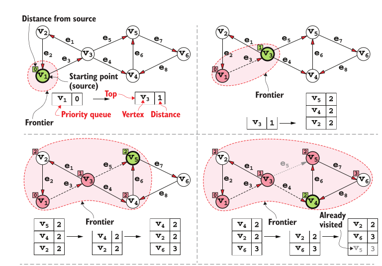• ?t=1716990255951 (View Highlight)
  • Note: Breadth-first search of a DAG
• How can we be sure that u is going to be visited in the right order, that is, after all vertices closer to the source than u and before the ones further away than u? This can be proved by induction on the distance of vertices. The base of the induc- tion is the initial case. We add the source vertex with a distance 0. This vertex is the only one at distance 0, and so any other vertex added later can’t be closer than (or as close as) the source. (View Highlight)
• For the inductive step, we assume that our hypothesis is true for all vertices at dis- tance d-1, and we want to prove it for vertex v at distance d; therefore, v is extracted (View Highlight)
• from the queue after all vertices at distance d-1 and before all vertices at distance d+1. From this, it follows that none of the vertices in the queue can have distance d+2, because no vertex at distance d+1 has been visited yet, and we only add vertices to the queue when examining each visited vertex’s adjacency list (so, the distance of a vertex added can only grow by 1 unit with respect to its parent). In turn, this guarantees that u will be visited before any vertex at distance d+2 (or further away) from the source. (View Highlight)
• we can obtain a tree considering the “parent” relation between visited and discovered vertices: each vertex u has exactly one parent, the vertex v that was being visited when u was discovered (line #15 in list- ing 14.2). This tree contains all the shortest paths from the source vertex to the other verti- ces, (View Highlight)
• ” It’s like when you are in a maze looking for the exit: you keep going as far away from the source as possible, choosing your direction at each intersection, until you hit a dead end (in graph terms, until you get to a vertex without any untraveled outgoing edges). At that point, you retrace your steps up to the previous bifurcation (the previous vertex with at least an untraveled edge), and choose a different path. This is the idea behind Depth First Search (DFS), (View Highlight)
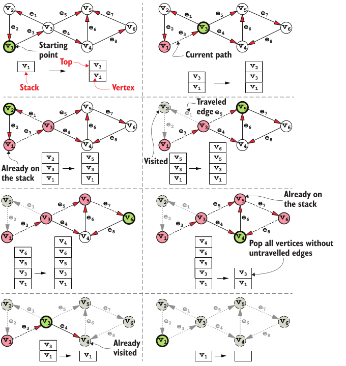• (View Highlight)
  • Note: Depth-first search
• their basic version, performing only the traversal, can be rewritten as the same templated algorithm where newly dis- covered vertices are added to a container from which, at each iteration, we get the next element. For BFS, this container will be a queue and we’ll process vertices in the order they are discovered, while for DFS, it will be a stack (implicit in the recursive version of this algorithm), and the traversal will try to go as far as possible before back- tracking and visit all vertex’s neighbors. (View Highlight)
• we can use the same algo- rithm shown in listing 14.3 to reconstruct the shortest path for Dijkstra’s as well (View Highlight)
• While in BFS each vertex was added to the (plain) queue and never updated, Dijks- tra’s algorithm uses a priority queue to keep track of the closest discovered vertices, and it’s possible that the priority10 of a vertex changes after it has already been added to the queue. (View Highlight)
• The best theoretical result is obtained with a Fibonacci heap, for which the amortized time to decrease the priority of an element is O(1). However, this data structure is complicated to implement and inefficient in practice, so our best bet is using heaps. (View Highlight)
• Dijkstra’s algorithm (like BFS) is a greedy algorithm, a kind of algorithm that can find the solution to a problem by making locally optimal choices. (View Highlight)
• To cope with negative edges, we need to use Bellman-Ford’s algorithm, an ingenious algorithm that uses the dynamic programming technique to derive a solution that takes into account negative-weight edges. Bellman-Ford’s algorithm is more expensive to run than Dijkstra’s; its running time is O(|V|*|E|). Although it can be applied to a broader set of graphs, it too has some limitations: it can’t work with graphs with negative-weight cycles11 (at the same time, though, it can be used as a test to find such cycles). (View Highlight)
• A* (View Highlight)
  • Note: This is not explained here in enough detail to actually use it.
• BFS and Dijkstra’s algorithms are very similar to each other; it turns out that they both are a particular case of the A* (pronounced “A-star”) algorithm. (View Highlight)