Chaudhury 2024, ch. 2 (linear algebra)

Notes from Chaudhury, et al. (2024), chapter 2

Highlights

• Sometimes the dot product is also referred to as inner product, denoted  a, b . Strictly  speaking, the phrase innerproduct is a bit more general; it applies to infinite-dimensional vectors as well. (View Highlight)
• A matrix with m rows and p columns, say Am,p, can be multiplied with another matrix with p rows and n columns, say Bp,n, to generate a matrix with m rows and n columns, say Cm,n: for example, Cm,n = Am,p Bp,n. Note that the number of columns in the left matrix must match the number of rows in the right matrix. Element i , j of the result matrix, Ci , j , is obtained by point-wise multiplication of the elements of the ith row vector of A and the jth column vector of B. (View Highlight)
• Given two matrices A and B, where the number of columns in A matches the number of rows in B (that is, it is possible to multiply them), the transpose of the product is the product of the individual transposes, in reversed order. (View Highlight)
• Thus the total error over the entire training dataset is obtained by taking the difference between the output and the ground truth vector, squaring its elements and adding them up. (View Highlight)
• That happens to be the definition of the squared magnitude or length or L2 norm of a vector: the dot product of the vector with itself. (View Highlight)
• Given any vector v, the corresponding unit vector can be obtained by dividing every element by the length of that vector. (View Highlight)
• a · b= aT b= a bcos (휃) for all dimensions (View Highlight)
• If the vectors have the same direction, the angle between them is 0 and the cosine is 1, implying maximum agreement. (View Highlight)
• If the angle between them is 180◦, the cosine is −1, implying that the vectors are anti-correlated. (View Highlight)
• The dot product between two vectors is also proportional to the lengths of the vectors. This means agreement scores between bigger vectors are higher (an agreement between the US president and the German chancellor counts more than an agreement between you and me). (View Highlight)
• Two vectors are orthogonal if their dot product is zero. Geometrically, this means the vectors are perpendicular to each other. Physically, this means the two vectors are independent: one cannot influence the other. (View Highlight)
• (View Highlight)
  • Note: Definition of a vector normal to the vector
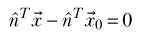
• The normal to the plane is the same at all points on the plane. (View Highlight)
• the line joining a known point x0 on the plane and any other arbitrary point x on the plane is at right angles to the normal ˆn. (View Highlight)
• During training, we are learning the weights and biases—this is essentially learning the orientation and position ofthe optimal plane that will separate the training inputs. (View Highlight)
• Given a set of vectors     v1, v2, …. vn, their span is defined as the set of all vectors that are linear combinations of the original set . (View Highlight)
• A set of vectors (points) in n dimensions form a vector space if and only if the operations of addition and scalar multiplication are defined on the set. In particular, this implies that it is possible to take linear combinations of members of a vector space. (View Highlight)
• Any pair of linearly independent vectors forms a basis in ℝ2. (View Highlight)
• Exactly n vectors are needed to span a space with dimensionality n. (View Highlight)
• the largest size of a set of linearly independent vectors in an n-dimensional space is n. (View Highlight)
• A set of vectors is said to be closed under linear combination if and only if the linear combination of any pair of vectors in the set also belongs to the same set. (View Highlight)
• The class of transforms that preserves collinearity are known as linear transforms. They can always be represented as a matrix multiplication. Conversely, all matrix mul- tiplications represent a linear transformation. (View Highlight)
• A function 휙 is a linear transform if and only if it satisfies 휙 훼a + 훽 b = 훼휙 a + 훽 휙 b ∀훼, 훽 ∈ℝ (View Highlight)
• Linear transform means transforms oflinear combinations are same as linear combinations oftransforms. (View Highlight)
• infinite-dimensional vectors (View Highlight)
  • Note: An example of a vector with infinite dimensions is a function space, such as the set of all real-valued continuous functions of f: [0, 1] \mapto \mathbb{R}. Each component is a real number on the interval [0, 1]. There is a well-defined concept of collinearity, multiplication, etc.
• linear transforms that operate on infinite-dimensional vectors are not matrices. But all linear transforms that operate on finite-dimensional vectors can be expressed as matrices. (View Highlight)
• Atensor may be viewed as a generalized n-dimensional array—although, strictly speaking, not all multidimensional arrays are tensors. (View Highlight)
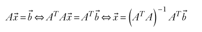
• The solution of Ax= b is x= A−1 b, a , a ≠ 0. where A−1 is the matrix inverse (View Highlight)
• A−1 exists if det (A) ≠ 0 (View Highlight)
• In fact, the following statements about the linear system Ax= b (with a square matrix) are equivalent: Matrix A has a row/column that can be expressed as a weighted sum of the others. Matrix A has linearly dependent rows or columns. Matrix A has zero determinant (such matrices are called singular matrices). The inverse of matrix A (i.e., A−1) does not exist. A is called singular. The linear system cannot be solved. (View Highlight)
• numerically unstable. Small changes in input cause the result to change drastically. (View Highlight)
• ill-conditioned. (View Highlight)
  • Note: An ill-conditioned linear system is one in which the determinant is close to, but not equal to, zero.
• Case 1: m > n (more equations than unknowns; overdetermined system) Case 2: m < n (fewer equations than unknown; underdetermined system) (View Highlight)
• There is no single set of values for the unknown that will satisfy all of them. (View Highlight)
• we have to find a solution that is optimal (causes as little error as possible) over all the equations. (View Highlight)
• we are looking for x such that Ax is as close to b as possible. (View Highlight)
• (View Highlight)
  • Note: Solving an overdetermined system using the pseudo-inverse .
• the pseudo-inverse of matrix A, denoted A+ =  ATA −1 AT. Unlike the inverse, the pseudo-inverse does not need the matrix to be square with linearly independent rows. Much like the regular linear system, we get the solution of the (possibly nonsquare) system of equations as Ax= b⇔ x= A+ b. (View Highlight)
• Ax is just a linear combination of the column vectors of A with the elements of x as the weights (View Highlight)
• The space of all vectors of the form Ax (that is, the linear span of the column vectors of A) is known as the column space of A. (View Highlight)
• The solution to the linear system of equations Ax= b can be viewed as finding the x that minimizes the difference of Ax and b: that is, minimizes Ax− b. This means we are trying to find a point in the column space of A that is closest to the point b. (View Highlight)
• In the friendly case where the matrix A is square and invertible, we can find a vector x such that Ax becomes exactly equal to b, which makes Ax− b = 0. (View Highlight)
• Ax− b ≤ Ay− b ∀y ∈n (View Highlight)
  • Note: Generalization of the solution for of , regardless of the dimension of .
• l try to find x such that Ax is closer to b than any other vector in the column space of A. Mathematically speaking,4 Ax− b ≤ Ay− b ∀y ∈n (2.19) (View Highlight)
• The solution vector x to equation 2.19 that we are looking for should correspond to the projection of b on the column space of A. This in turn means b− Ax is orthogonal (perpendicular) to all vectors in the column space of A (see figure 2.12). (View Highlight)
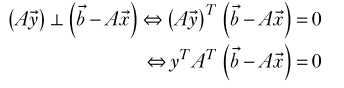• (View Highlight)
• For the previous equation to be true for all vectors y, we must have AT b− Ax = 0. (View Highlight)

New highlights added June 19, 2024 at 2:30 PM

• a typical linear transform leaves a few points in the space (almost) unaffected. (View Highlight)
• The axis of rotation is an eigenvector of the rotation transformation. (View Highlight)
• if e is an eigenvector of the square matrix A,5 then Ae=휆 (View Highlight)
• det (A−휆I) =0 (View Highlight)
• A rotation matrix will always have 1 as an eigenvalue. The corresponding eigenvector will be the axis ofrotation. In 3D, the other two eigenvalues will be complex numbers yielding the angle ofrotation. (View Highlight)
• Two eigenvectors of a symmetric matrix that correspond to different eigenvalues are mutually orthogonal. (View Highlight)
• A matrix A is symmetric if AT = A. (View Highlight)
• A matrix R is orthogonal if and only if it its transpose is also its inverse: that is, RTR = RRT = I. All rotations matrices are orthogonal matrices. All orthogonal matrices represent some rotation. (View Highlight)
• Orthogonality implies that rotation is length-preserving. Given any vector x and rotation matrix R, let y =Rx be the rotated vector. The lengths (magnitudes) of the two vectors x, y are equal since it is easy to see that y = yTy =  Rx T  Rx = xTRTRx= xTIx= xT x=  x  (View Highlight)
• Negating the angle of rotation is equivalent to inverting the rotation matrix, which is equivalent to transposing the rotation matrix. (View Highlight)
• AS =SΛ (View Highlight)
  • Note: is a square matrix is the matrix of its eigenvalues is the diagonal matrix of eigenvalues corresponding to X And we reach this finding by expressing the definition of an eigenvalue in matrix form.
• which leads to A=SΛS−1 and Λ=S−1AS (View Highlight)
• SΛST x= b where S is the matrix with eigenvectors of A as its columns: S =  e1 e2 · · · en  (View Highlight)
  • Note: Since we can obtain the eigenvalues and eigenvectors of a matrix numerically, we can solve for by using the diagonalization in place of . Solving with diagonalization replaces matrix inversion (necessary for direct solution) with a transpose and a matrix multiplication, which is much simpler.